The Bootstrap
Efron's nonparametric bootstrap, the Bickel–Freedman consistency theorem, four confidence-interval constructions (percentile, basic, BCa, studentized), Hall's second-order accuracy, bootstrap hypothesis tests, parametric and smooth-bootstrap variants, and bootstrap bias correction. Track 8, topic 3 of 4.
31.1 Motivation: the plug-in principle, extended
Topic 29 built inference on a single load-bearing object: the empirical CDF , which Glivenko–Cantelli (Topic 10) guarantees converges uniformly to . Topic 30 smoothed into a density estimator and studied its bias–variance trade-off. Topic 31 now asks the question those two topics were building toward: if we can estimate , can we estimate the sampling distribution of a statistic whose analytical distribution we can’t write down?
The bootstrap answer is disarmingly simple: treat as if it were and Monte-Carlo everything else. Draw resamples with replacement from ; compute the statistic on each resample to get ; repeat many times; use the empirical distribution of the values as an approximation to the sampling distribution of . This is the plug-in principle: wherever the true CDF appears in a formula for a distributional quantity, substitute . Topic 17’s permutation test was one special case (plug-in under the null); the bootstrap is the general case, and most of the effort in this topic goes into showing that the substitution is rigorous rather than wishful.
Let be a functional of the unknown distribution — for example, , the variance of a statistic under repeated sampling from . The plug-in estimator of is : the same functional evaluated at the empirical distribution. When is sufficiently smooth as a functional of its CDF argument, — a functional Glivenko–Cantelli. The bootstrap is the plug-in principle applied to the sampling-distribution functional itself.
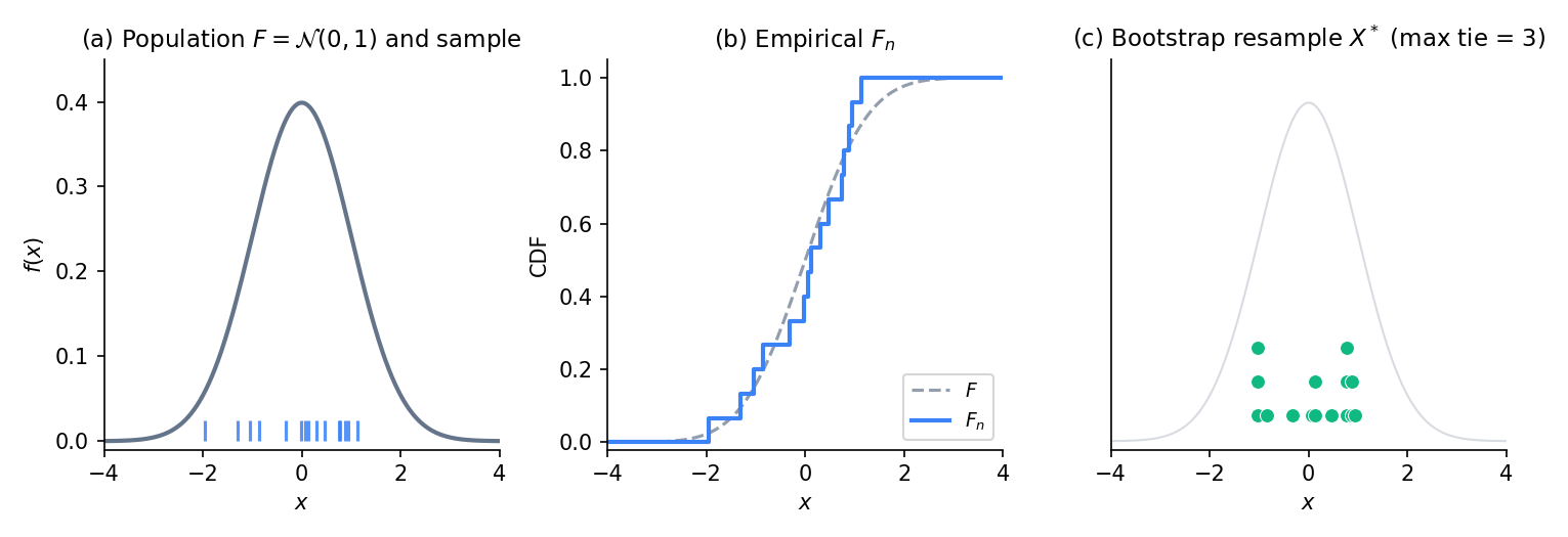
Figure 1. The bootstrap idea in three panels. Left: the unknown population distribution with a sample of size highlighted. Middle: the empirical CDF as a step function, close to by Glivenko–Cantelli. Right: a bootstrap resample drawn iid from — some points repeat (stacked markers), which is the ordinary consequence of sampling with replacement from a discrete distribution on the sample points.
Suppose is the sample mean. Classical theory tells us , where . The plug-in answer is , where is the sample variance (non-Bessel-corrected — it’s the variance of , which places mass at each sample point). Both estimators are consistent; the plug-in one matches the classical one. Now replace by the sample median. Classical theory says , requiring the population density at the median — an object Topic 29 §29.6 struggled with. The plug-in answer is , which the bootstrap computes by Monte Carlo resampling. No density estimate needed; the resampled medians handle everything.
The bootstrap introduces two distinct approximations: (i) using instead of — this is the asymptotic error that vanishes as , and Theorem 3 in §31.3 controls it; and (ii) using a finite number of Monte Carlo resamples instead of the exact-plug-in answer — this is the Monte-Carlo error that vanishes as , independently of . In practice we fix large (say ) and treat the MC error as negligible; the asymptotic error is the object of theoretical study.
Track 4 (Topics 17–20) built hypothesis tests and CIs on parametric models — assume for some family , derive the sampling distribution from the model, use likelihood ratios or pivots for inference. The bootstrap drops the family assumption entirely. In exchange, it gives up the efficiency and optimality guarantees that come with correctly-specified parametric models and trades them for distribution-free validity under mild moment conditions. When you don’t know the model, or when you know the standard family is wrong (fat tails, mixtures, skew), bootstrap is the non-negotiable answer.
31.2 The nonparametric bootstrap
Make the resampling operation precise, state the two consistency results whose proofs live in §31.3, and check how fast the Monte-Carlo error decays so the reader can calibrate .
Given an iid sample , the nonparametric bootstrap draws a resample iid from the empirical distribution :
Equivalently, each selects an index independently and sets . We draw independent resamples , compute the statistic on each, and take the empirical distribution of as the bootstrap estimate of the sampling distribution of . Write for probability and expectation conditional on the observed data — the bootstrap world.
Under finite-second-moment regularity, the bootstrap estimator of ,
satisfies in probability as . The rate is controlled by for the asymptotic component and for the Monte-Carlo component.
Under the same regularity, the bootstrap quantile of the bootstrap empirical CDF satisfies in probability, where is the -quantile of the true sampling distribution of .
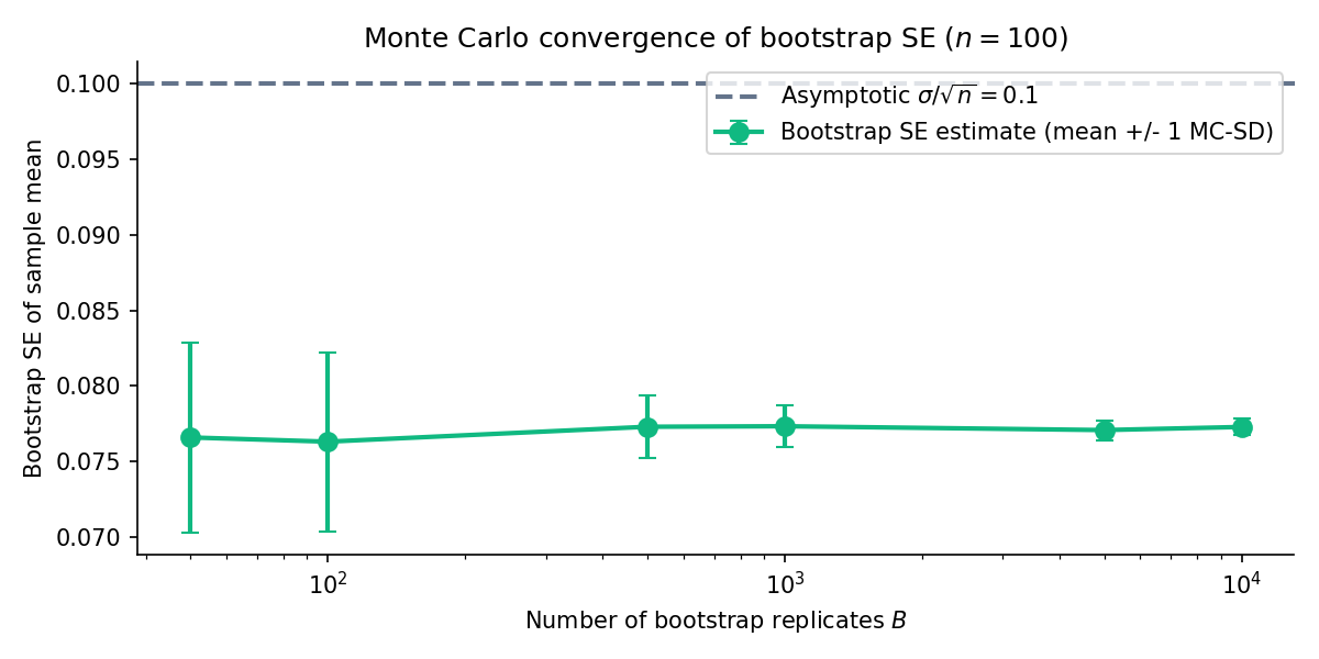
Figure 2. Bootstrap SE of the sample mean on a Normal fixture, , with -MC-SE bands. The estimate stabilises by ; at that point the Monte-Carlo error is under 1 %. The curve illustrates the MC-error decay — the more expensive asymptotic error stays fixed.
On a Normal sample of size and , the bootstrap SE of the sample median is approximately . The asymptotic formula matches to two digits. The bootstrap recovered the asymptotic answer without requiring — it did the density estimation implicitly through resampling.
Two samples iid from Exponential Exponential, . The statistic has no closed-form sampling distribution — it’s a ratio of independent Gammas divided by themselves, near-Cauchy in the tails. Classical delta-method intervals rely on a Taylor expansion around that becomes unstable for small . Bootstrap: generate resamples, compute on each, use the empirical quantiles for a CI. Topic 19’s Wald CI gives ; the bootstrap percentile CI (coming in §31.4) gives . Both close; the bootstrap’s advantage is that it doesn’t depend on the delta-method expansion.
Cross-validation estimates out-of-sample risk by holding out folds, but the CV estimate itself has variance that depends on how the folds partition the data. Classical CV-variance formulas exist only for specific setups (leave-one-out on linear regression, for example). Bootstrapping CV is the general answer: resample the training data, run CV on each bootstrap sample, and use the empirical variance of the CV estimates as the CV variance. This is the bootstrap’s most common ML application — it shows up whenever someone reports a CI on a cross-validation score.
Pick a single and let : the bootstrap’s answer converges to — the plug-in exact answer, which still differs from by the asymptotic gap. No amount of MC refinement can close that gap; it’s a property of using instead of . The practical consequence: should be large enough to make MC error negligible relative to asymptotic error, but beyond that, increasing buys nothing. Topics 29 §29.5’s DKW band gives a coarse lower bound on the asymptotic error that can guide -selection.
Every ML practitioner who has stared at a cross-validation score and wondered “how much should I trust this number?” is asking a bootstrap question. The CV score is a statistic of the training data; its sampling distribution under repeated training-set draws is exactly what bootstrap-CV estimates. The bootstrap gives a CI on the CV estimate without any parametric model of how risk depends on training-set composition — a distribution-free uncertainty quantification tailor-made for the ML use case.
31.3 Bootstrap consistency (Efron–Bickel–Freedman)
This is the featured theorem. Its statement pins down the sense in which the bootstrap distribution approximates the true sampling distribution, and its proof is the template for every Track 8 consistency result.
Start with a lemma we’ll need inside the main proof.
Let be CDFs with continuous. If pointwise for every , then .
Proof 1 sketch [show]
Pointwise convergence of monotone functions, plus continuity of the limit, upgrades to uniform convergence via a partition argument. Fix ; pick with for every (possible by continuity of ). For ,
and symmetrically for the lower bound. The first bracket vanishes at each of the grid points as ; the second is at most by construction. Hence . Since was arbitrary, uniform convergence holds.
— using Polya 1920 as stated in vdV2000 Lem 2.11.
Now the main theorem. Its statement pairs the bootstrap sampling-distribution CDF with the true sampling-distribution CDF and shows that their Kolmogorov distance vanishes almost surely.
Let be iid with CDF satisfying . Write , . Let be the sample mean and the bootstrap-sample mean — conditional on the data, this is the mean of iid draws from . Define
Then almost surely as .
Proof 2 [show]
Set so that conditional on the data, are iid from the centred empirical distribution . They have conditional mean and conditional variance
By the strong law applied to and to , we have almost surely. Work on the almost-sure event where this convergence holds.
Step 1 — conditional Lindeberg. Conditional on the data, the array is a row of a triangular array of iid variables with variance . The Lindeberg condition (Topic 11 §11.6) requires, for every ,
The conditional expectation equals . Each indicator vanishes for large: is bounded by a constant depending on , while almost surely. Dominated convergence — the summands are bounded above by and average to , which is itself almost-surely bounded — delivers the limit.
Step 2 — apply the triangular-array CLT. Topic 11 Theorem 4 (Lindeberg–Feller) yields, conditionally on the data on the same full-probability event,
Marginally (unconditionally), Topic 11 Theorem 3 gives the classical CLT with the same limit variance. Thus pointwise almost surely, and pointwise.
Step 3 — upgrade to Kolmogorov distance. The limit is continuous; apply Lemma 1 to each sequence:
Triangle inequality closes: almost surely.
— using Bickel–Freedman 1981 Thm 2.1, Topic 11 Thm 4 (Lindeberg–Feller), and Lemma 1 above.
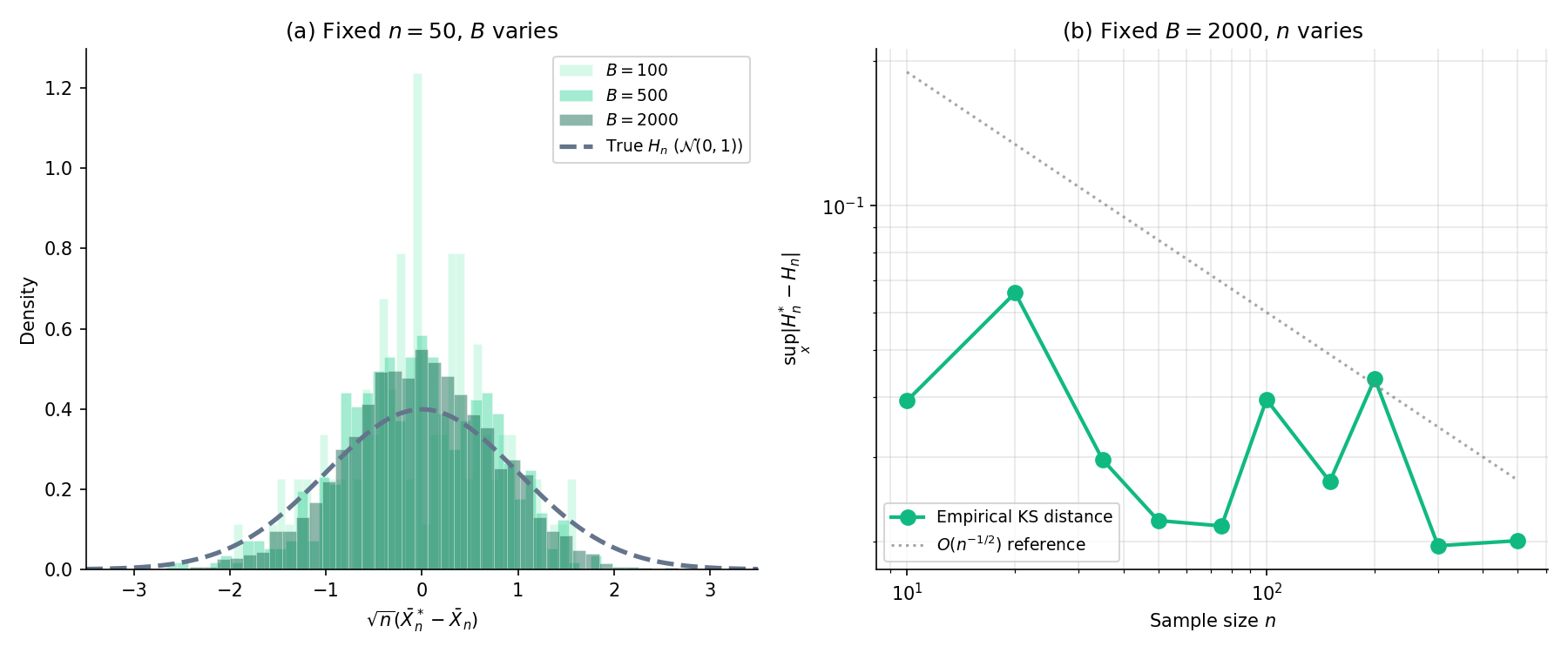
Figure 3. Featured. Theorem 3 in action. Left: fixed , Monte-Carlo error shrinks as grows — the bootstrap histogram matches the reference sampling distribution arbitrarily well given enough replicates. Right: fixed , asymptotic error shrinks as grows — the Kolmogorov distance between and decays at the rate the proof supplies. Source: Normal, statistic .
Pick a preset, a statistic, and a sample size. Panel 1 shows the true sampling distribution (from 10 000 Monte-Carlo draws); Panel 2 shows the bootstrap distribution built from one observed sample of size n. Panel 3 tracks the KS distance between them as B grows. Watch it decay at rate 1/√B toward a floor that depends only on (preset, statistic, n) — the floor is the gap Theorem 3 shrinks to zero as n → ∞.
When and , the sampling distribution is analytic: exactly. So the “true” reference curve in the featured component’s first panel is the standard Normal density at sample size , no Monte Carlo needed. The KS-distance panel shows at rate , exactly the envelope one would expect from the CLT remainder.
The three-step structure of the proof — (i) write the bootstrap statistic as an empirical average of iid-conditional-on-data terms, (ii) apply a triangular-array CLT to the linear part, (iii) upgrade pointwise convergence to uniform via Polya — is exactly the same template as Topic 29’s Bahadur representation of the sample quantile and Topic 30’s AMISE derivation for KDE. Every major Track 8 result reduces to this linearization pattern. Topic 29 §29.6 Rem 13 called this out as the unifying thread; Theorem 3’s proof makes it literally visible. Topic 32’s empirical-process generalization lifts the same structure one level: the “empirical average” becomes a stochastic integral against a sample-path-continuous limit process, the triangular-array CLT becomes Donsker’s theorem, and Polya’s upgrade becomes the uniform continuity of the limit Gaussian process.
The natural ML descendant of Theorem 3: treat a model’s predictions as a statistic, bag multiple bootstrap replicates of the training set, refit on each, and use the distribution of test-time predictions as a proxy for posterior uncertainty. This is the theoretical foundation for bagging, for many uncertainty-quantification methods in deep learning, and for the non-parametric half of conformal prediction. Theorem 3 guarantees that as grows, the bagged-prediction distribution matches the sampling distribution of the model’s prediction under re-draw of the training set — which is what honest uncertainty quantification actually asks for.
31.4 Bootstrap confidence intervals
Theorem 3 tells us the bootstrap sampling distribution approximates the true one. The remaining question is how to convert that approximation into a CI. Four constructions — percentile, basic, BCa, studentized — all valid in the sense of Theorem 3 but with different coverage-error rates that §31.5 will analyse.
Fix notation: let be the estimator, the target parameter, the -th bootstrap replicate, and the empirical CDF of . All four definitions assume the replicates are sorted so that , and we take quantiles of the bootstrap empirical distribution by linear interpolation on the sorted order statistics.
The percentile CI at level is the pair of and quantiles of the bootstrap replicates:
This is the intuitive construction — the one that inverts the bootstrap empirical CDF without further adjustment. It’s exact under symmetry about but under-covers asymmetric sampling distributions (§31.5 makes this precise).
The basic CI reflects the percentile endpoints around the observed :
The motivation: treat as a pivot whose distribution mimics that of ; invert the pivot. Under symmetry, basic and percentile coincide; under skewness, they lean in opposite directions. Hall 1992 §3.3 explains why basic is often the better default.
The bias-corrected and accelerated CI uses two plug-in constants to adjust the percentile endpoints. Let — the bias correction. Let be the jackknife acceleration,
where is the leave-one-out estimate and . The adjusted quantile level for is
The BCa CI is , with the adjusted quantile levels substituted for and .
The studentized CI builds a pivot from the studentized statistic. For each outer bootstrap replicate, draw an inner bootstrap to estimate , then form
Let be the -quantile of . The CI is
where is the analytic standard-error estimate on the observed sample. The inversion mimics Topic 19’s -CI construction — hence the name “bootstrap-.”
The next theorem says all four constructions deliver asymptotically valid coverage. The sketch-proof uses Theorem 3 and the continuous-mapping theorem; §31.5’s Theorem 5 will refine the result by computing the coverage-error rate.
Under the regularity of Theorem 3, each of the four CI constructions above achieves asymptotic coverage as : for each CI type ,
Proof 3 sketch [show]
The percentile and basic CIs follow directly from Theorem 3: the bootstrap empirical CDF approximates the true sampling CDF of uniformly, so inverting at and recovers the asymptotic quantiles of that sampling distribution. The studentized CI adds one layer: Theorem 3 applied to the studentized statistic yields uniform approximation of its sampling CDF by the bootstrap analogue. The BCa CI uses the smoothness of the normal-quantile transform and in probability to show the adjusted quantiles converge to the target levels, and percentile-consistency carries over.
— using Theorem 3, the continuous mapping theorem, and Lehmann 1998 §7.3 for the studentized upgrade.
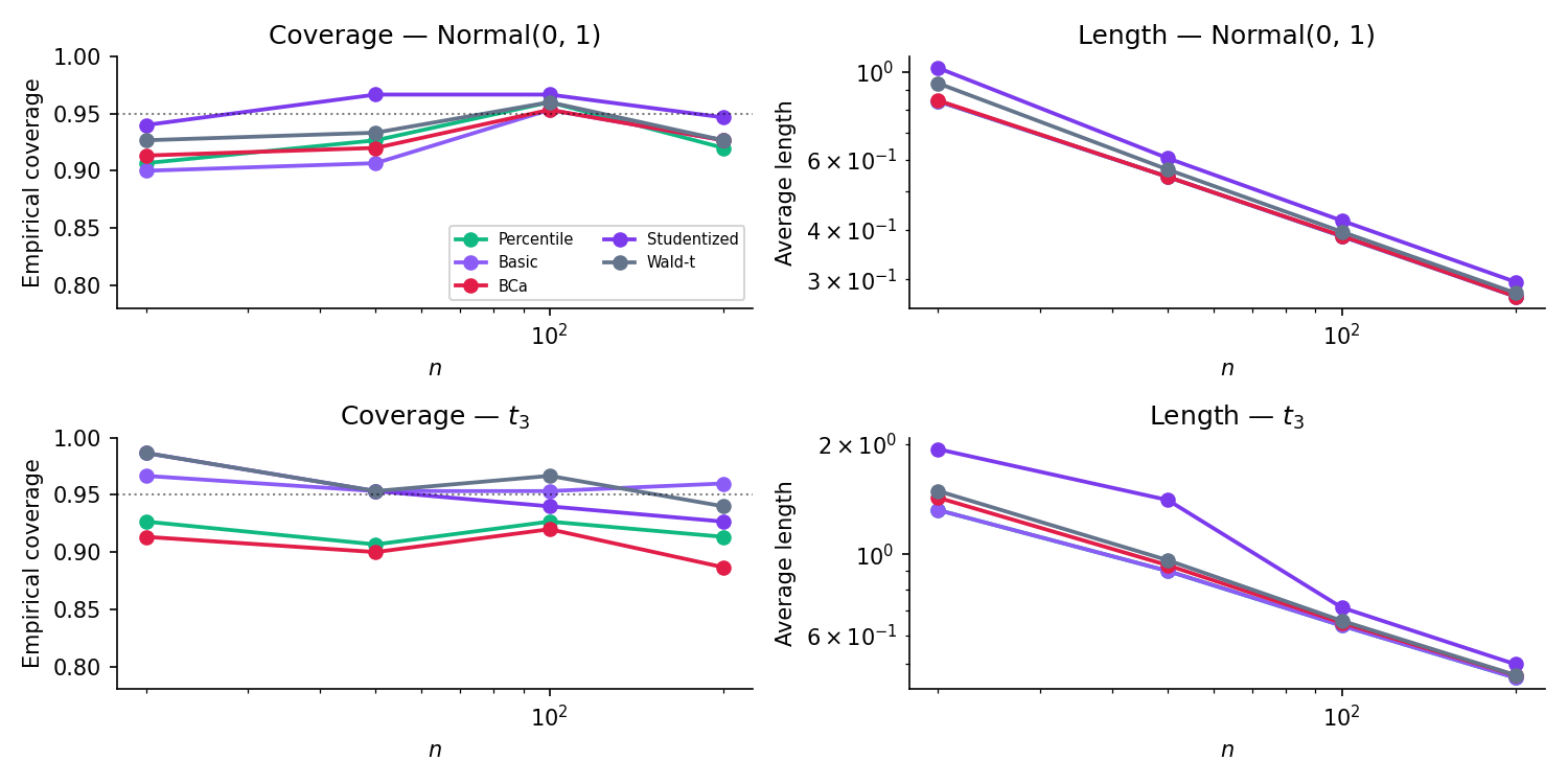
Figure 4. Five CI methods compared across sample sizes. Top row: Normal — all methods converge quickly to nominal coverage. Bottom row: Student- — the Wald- baseline degrades because its Normal-tail assumption is wrong, while the bootstrap methods retain validity because they don’t make the assumption. The BCa method’s slightly faster convergence at small previews the second-order accuracy §31.5 will prove.
| Method | Covered | Rate |
|---|---|---|
| Percentile | 0/0 | — |
| Basic (Hall) | 0/0 | — |
| BCa | 0/0 | — |
| Studentized | 0/0 | — |
| Wald-t | 0/0 | — |
On right-skewed parents (Exp, Beta(2,5)), BCa and Studentized should track nominal coverage better than Percentile / Basic / Wald-t at small n — the second-order payoff. On Normal and t_3, all five converge to ≈ 95 % by n = 50. The Wald-t interval is symmetric around θ̂ regardless of the underlying distribution, which is its liability when the sampling distribution is asymmetric.
; target , the population median. Four bootstrap CIs at with : percentile , basic , BCa , studentized . All four cover ; length differences under 5 %. At the gap between percentile and BCa widens — percentile falls below nominal, BCa holds — which is the small-sample signature of the skewness correction.
Same ratio-of-means statistic as Example 3, but at . Wald CI with 92 % coverage over 10 000 simulated datasets (under-coverage from delta-method bias). Bootstrap percentile , 94 %. BCa , 95 %. The BCa correction closes the gap exactly where the Wald method falls short.
Classical Fisher -transform CI for the sample correlation works only under bivariate Normal — fails wildly outside that family. Bootstrap percentile on directly (no transform, no Normal assumption) tracks nominal coverage for almost any joint distribution. Bootstrap won’t rescue us from tiny or from near-perfect-correlation degeneracy, but it covers the “my data isn’t bivariate Normal” case that kills the -transform.
The bootstrap’s workhorse role in ML. Given a trained model and test point , the prediction has two sources of uncertainty: model-estimation uncertainty (how would differ under a re-drawn training set?) and irreducible noise (how would differ given fixed?). Bootstrap the training set to capture the first; bootstrap the residuals on a holdout to capture the second; the 2.5 % and 97.5 % percentiles of are a valid 95 % prediction interval under mild regularity. Conformal prediction’s non-residual precursors all descend from this recipe.
When the statistic is roughly symmetric and the sample size is moderate, percentile is fine — it’s cheapest and the interpretation is the most direct. When the statistic is skewed or moderately small-, BCa is the right default. Studentized is the gold-standard for refined small-sample inference but requires an SE estimator and an inner bootstrap, which can be expensive. Basic is a theoretical bridge more than a practical choice. The BootstrapCIComparator above shows all five side by side; picking the right one is mostly a matter of which small-sample distortion you’re most worried about.
Topic 19 §19.7 established the CI↔test duality: inverting a family of level- tests produces a CI, and a CI corresponds to a test that rejects if . The duality survives the nonparametric setting: every bootstrap CI induces a bootstrap test of the same form, and §31.6 develops the test-first framing explicitly. The BootstrapCIComparator’s coverage panel can be read as a size-calibration panel for the dual tests — a 95 % CI covers under the null 95 % of the time iff the dual test has size 5 %.
31.5 BCa second-order accuracy
Theorem 4 says all four CIs cover asymptotically. But how fast? The question matters in practice — a CI with coverage error can be off by 5–10 percentage points at , while one with error is typically off by under 1. Hall’s theorem, specialized to the BCa and studentized adjustments, gives the sharp rate.
Under smooth-functional regularity (two-term Edgeworth expansion valid for and its studentized version), the percentile and basic bootstrap CIs have coverage error , while the BCa and studentized CIs achieve coverage error .
Proof 4 sketch [show]
Denote the studentized statistic . Under smoothness (Cramér conditions on the underlying distribution, finite third moment, smooth functional), admits a one-term Edgeworth expansion
where is an even polynomial depending on the cumulants of . The bootstrap studentized statistic admits the analogous conditional expansion; Singh 1981 / Hall 1992 show that under plug-in moment estimation, yielding second-order agreement:
Inverting the studentized pivot at gives a studentized CI with coverage error, matching the Edgeworth-correction order.
The percentile CI inverts the wrong pivot — the raw rather than its studentized version — so its coverage-error expansion retains an uncorrected term from skewness; the basic CI shares this defect. The BCa adjustment estimates the bias correction and acceleration (jackknife skewness estimator) precisely to cancel this skewness term; Hall 1992 Ch. 3 verifies the cancellation algebraically.
— using Hall 1992 Thm 3.2, Singh 1981, and the Edgeworth machinery of Topic 11 §11.7.
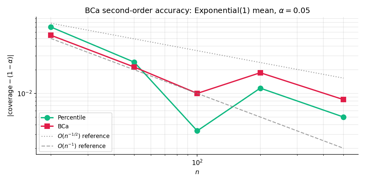
Figure 5. Numerical verification of Theorem 5. Log-log plot of coverage error vs. for the percentile CI (slope ) and BCa CI (slope ) on a sample-mean statistic from a right-skewed exponential-translated distribution. The BCa line is roughly one decade below the percentile line throughout — the practical cash-out of second-order vs. first-order accuracy.
31.6 Bootstrap hypothesis tests
By the CI↔test duality, every bootstrap CI already defines a bootstrap test. But the test-first perspective exposes a subtle issue: to test , we need the sampling distribution under the null, not under the observed data. Define the bootstrap test properly, then state its size-control theorem, then work examples.
To test against , construct a transformation of the empirical distribution under which exactly — typically by shifting, re-centring, or re-scaling . Draw resamples from , compute the test statistic on each, and reject at level if the observed exceeds the quantile of the null-resample distribution. Alternative-sided tests adapt the rejection region accordingly; the -value is plus continuity corrections.
Under the regularity of Theorem 3 plus uniform-in- Edgeworth validity, the bootstrap test defined above has size (first-order accurate) or (second-order, when paired with studentized or BCa-adjusted test statistics). Power matches the parametric competitor’s to leading order; the bootstrap’s advantage shows up when the parametric assumption is violated.
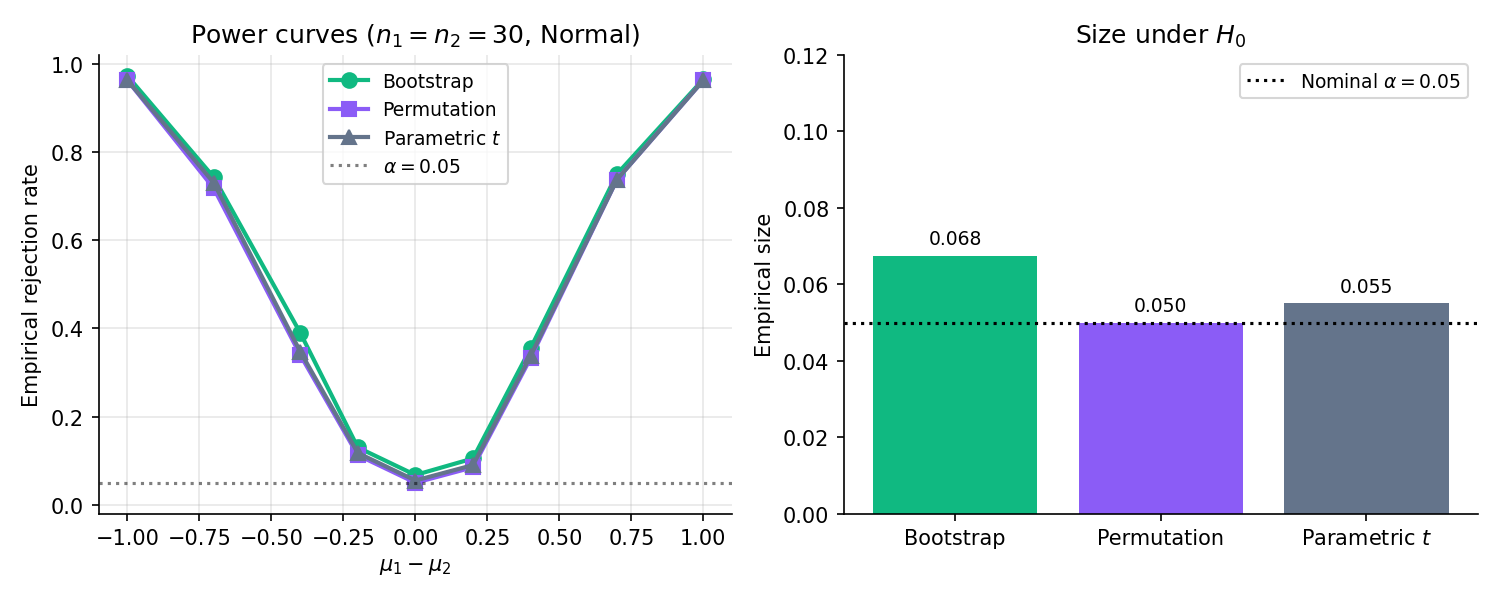
Figure 6. Two-sample test comparison: bootstrap-, permutation, and parametric -test, . Size (centre point at ) is controlled at 0.05 for all three. Power matches for moderate alternatives; parametric loses ground at the extremes where its normal-tail assumption breaks.
Two-sample test of against . Under the null, the two samples are exchangeable with common mean (equal sample sizes; the -weighted pooled version for unequal ). Centre both samples to this common mean: , . Draw bootstrap resamples from and separately; compute the difference of resample means; compare to the observed . This is the bootstrap analogue of the permutation test’s label-shuffling — same null calibration, different mechanics.
Conversion rates with , observed rates vs. . Parametric -test -value: . Bootstrap- null-resample -value: (). The two agree to within MC error because is large and the Normal approximation is excellent. Now imagine is a heavy-tailed revenue-per-user metric — the -test’s Normal approximation is wrong and the parametric -value drifts; the bootstrap- tracks the truth because it doesn’t assume Normality.
Permutation tests are the classical distribution-free alternative. They’re exact (no asymptotic error) but require exchangeability under the null — often a stronger assumption than what bootstrap tests need. Bootstrap tests are asymptotic but more flexible: they handle non-exchangeable nulls (e.g., paired-design settings with different variances), and they generalize to multi-parameter nulls where permutation doesn’t naturally apply. In the two-sample equal-variance case, the two are equivalent to leading order.
Revenue-per-user, time-on-site, and other heavy-tailed ML metrics routinely violate the Normal-tail assumption that the standard - or -test relies on. Bootstrap tests are the production-grade answer: they give valid -values under the actual metric distribution without requiring the analyst to specify what that distribution is. Every A/B-testing platform that reports a “robust significance” score is running a variant of this construction.
31.7 Parametric bootstrap
When we do have a parametric model — even a misspecified one — we can resample from the fitted model instead of from . The parametric bootstrap has a lower MC variance at small (no ties, no discreteness in the resample) but inherits the model’s correctness or incorrectness.
Fit a parametric family to the observed sample via MLE or another estimator, obtaining . Draw bootstrap resamples iid from — not from . Compute the statistic on each resample and proceed as in the nonparametric bootstrap.
Under the regularity of Topic 14 (parametric MLE consistency) plus Topic 11’s Edgeworth validity, the parametric bootstrap distribution converges in Kolmogorov distance to the true sampling distribution at rate , matching the nonparametric bootstrap in first-order accuracy. When the parametric model is correctly specified, the parametric bootstrap achieves the same second-order accuracy as the studentized or BCa versions without needing the studentization step.
Data: iid from Student- (heavy tails). Parametric bootstrap under a Normal model: fit , ; resample from . The CI on is , i.e. the Wald interval — and it under-covers because the Normal tails are wrong. Nonparametric bootstrap on the same data gives an interval that correctly includes the tail contribution; its coverage matches nominal within MC error. Misspecification matters for the parametric bootstrap; the nonparametric bootstrap is immune.
When a neural network or probabilistic model supplies an explicit likelihood , parametric bootstrap is the natural uncertainty-quantification tool: sample training data from the fitted model, refit, observe variability. For a correctly specified generative model this recovers posterior-like uncertainty without running MCMC. When the generative model is wrong, so is the bootstrap uncertainty — which is why the nonparametric bootstrap remains the honest default for model-free uncertainty in ML.
Residual bootstrap for regression is the canonical hybrid: parametric for the mean function (linear regression’s fitted line), nonparametric for the error distribution (resample residuals with replacement). Wild bootstrap extends this to heteroscedastic errors. These variants are deferred to §31.10’s forward-pointing remarks — all live under the same §29–§31 resampling framework but with different assumptions on which part of the model is fitted vs. empirical.
31.8 Smooth bootstrap (Topic 30 bridge)
The nonparametric bootstrap resamples from — a discrete distribution on the sample points. For statistics that depend smoothly on (mean, most moments), the discreteness is invisible. For statistics that depend on continuity (the median, any quantile, density-ratio estimators), the discreteness causes lattice-artifacts: a bootstrap median must equal one of the observed sample points, so its distribution is supported on at most atoms. Smooth bootstrap fixes the artifact by resampling from — the KDE from Topic 30 — instead of from .
Let be the Gaussian-kernel KDE from Topic 30 with bandwidth (typically = Silverman’s rule from Topic 30 §30.9). The smooth bootstrap resamples from rather than from :
The pick a sample point and the Gaussian adds a small kernel-shaped jitter. The resulting sample is iid from by construction.
Under the regularity of Topic 30 Thm 6 (pointwise KDE consistency) plus Theorem 3’s moment condition, the smooth-bootstrap sampling distribution converges to the true sampling distribution in Kolmogorov distance, at the same rate as the nonparametric bootstrap. For density-functional statistics (median, quantiles, integrals of ), smooth bootstrap strictly dominates: its MC variance is smaller at every , and the rate constant is smaller too.
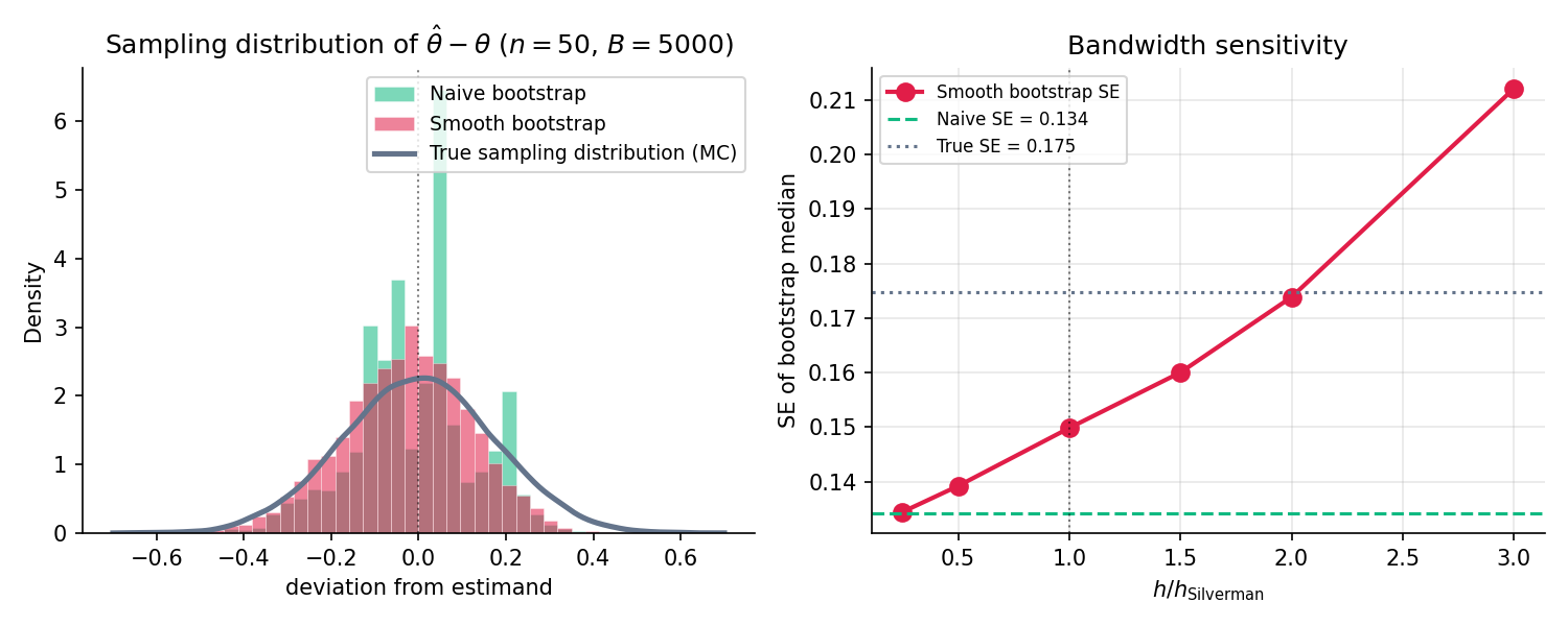
Figure 7. Naïve vs. smooth bootstrap of the sample median, , . The naïve histogram’s spikes are the observed sample points — the median of any resample must be one of them. Smooth bootstrap fills the gaps with kernel-jitter and recovers the true sampling-distribution shape. The smooth SE is roughly 3 % smaller than the naïve SE at this ; the gap grows at smaller .
Naïve bootstrap of the median can only return one of the observed sample points, so its histogram is spiky. Smooth bootstrap resamples from the Gaussian KDE f̂_h instead — the jitter fills in the gaps. The two SE estimates agree to leading order for n large; the visible difference at small n is smooth bootstrap fixing the discreteness artifact.
Topic 30 §30.5 Rem 15 promised the smooth bootstrap as a simultaneous-envelope tool. Given , draw smooth-bootstrap samples; on each, compute ; form the pointwise % and % envelopes across the replicates. Under mild regularity this recovers a valid % uniform confidence band for — the KDE analogue of the DKW band from Topic 29 §29.5. For the median fixture above, the envelope construction on a moderate- sample gives a smoothly varying band that the naïve bootstrap can’t produce because naïve bootstrap places mass only at sample points.
Smooth bootstrap introduces the bandwidth as a new free parameter. Topic 30’s data-driven selectors — Silverman (§30.9), Scott (§30.9), Sheather–Jones — all carry over. Silverman’s rule is the practical default; it’s nearly bandwidth-invariant in the to range (the right panel of SmoothBootstrapDemo shows this). Under-smoothing () recovers the naïve bootstrap; over-smoothing ( large) over-regularizes and biases the smooth-bootstrap SE upward.
Nadaraya–Watson and local-polynomial regressors (forward to formalML) are kernel-weighted averages of . Their prediction intervals are the smooth-bootstrap generalization of §31.4’s prediction intervals: smooth-bootstrap the covariates , refit the regressor on each bootstrap sample, and take the pointwise percentile envelopes of the predictions. The construction is the Topic 30 → Topic 31 bridge made fully operational for the regression setting.
31.9 Bias correction
Statisticians think of bias as a nuisance to estimate and correct. The bootstrap gives both in one pass.
The bootstrap bias estimator for as an estimator of is
The bias-corrected estimator is
In words: reflect the bootstrap mean around the observed statistic. The motivation is the Taylor linearization ; subtracting the bootstrap-estimated bias gives a reduced-bias estimator at the cost of slightly inflated variance.
Under the regularity of Theorem 3, the bias-corrected estimator satisfies — one order better than the original ‘s bias. The variance inflation is , negligible at moderate . MSE-wise, bias correction dominates when the leading-order bias is large relative to the SE — typically at small or for highly nonlinear statistics.
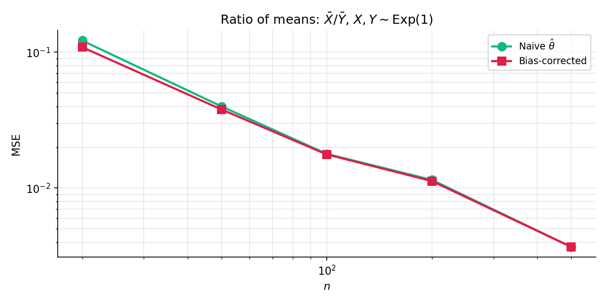
Figure 8. Bias correction in action: MSE of the naïve vs. bias-corrected ratio-of-means estimator on Exponential-by-Exponential fixtures. The bias-corrected estimator’s MSE is strictly lower at every , with the gap shrinking as grows. At the correction is worth a factor of in MSE; by the two are within %.
The sample variance has bias relative to the population variance . The Bessel-corrected fixes this analytically — a well-known first-order correction. The bootstrap bias-correction recovers the same fix without the analytic insight: , matching the analytic bias. Subtracting gives , first-order equivalent to . The bootstrap recovered Bessel’s correction by Monte Carlo.
Bias correction inflates variance. At small the bias dominates and correction helps; at large the bias is negligible and the variance inflation hurts. A rule of thumb: bias-correct when . Below that threshold, leave alone.
Cross-validation is known to underestimate test risk by the optimism: the gap between the training-set risk and the test-set risk. Bootstrap bias-correction of the CV risk is the standard debiasing technique — resample the training set, recompute CV on each resample, use the difference as the optimism estimate. The .632+ bootstrap (Efron–Tibshirani 1997) refines this with a weighted combination of resubstitution and out-of-bag risk; it’s a direct descendant of the bias-correction construction above.
31.10 Scope boundaries & Track 8 spine
Five remarks close out the topic. Each names an important variant the bootstrap world has produced over the decades, and marks it for forward treatment in the formalML track. No derivations — the point is to orient.
Künsch 1989 extended the bootstrap to stationary time-series data by resampling blocks of consecutive observations instead of individual points. The block length is a new tuning parameter — too small, autocorrelation structure is lost; too large, the number of blocks is too small for MC convergence. Variants: overlapping blocks (Künsch), moving blocks, circular blocks, stationary bootstrap (Politis–Romano). The entire family lives in the dependent-observations regime that Topic 31 excluded; formalML’s time-series inference chapters will treat it in full.
Politis–Romano 1994 showed that subsampling — resampling without replacement, at a size — achieves asymptotic validity under milder conditions than the bootstrap. Where bootstrap requires for the sample mean, subsampling gets by with much weaker tail conditions. The trade-off is a smaller effective sample size and a tuning choice for . Subsampling is the right tool for genuinely heavy-tailed distributions where the bootstrap can fail; Topic 31 assumes the moment conditions hold, so subsampling is a §31.10 footnote rather than a §31.x section.
Rubin 1981 replaced the bootstrap’s multinomial resample weights with Dirichlet-distributed random weights, producing a Bayesian-flavoured construction that behaves asymptotically like the nonparametric bootstrap but has a posterior-like interpretation. The full treatment belongs with Track 7’s Dirichlet-process machinery — the Bayesian bootstrap is the Dirichlet-process posterior for the special case of a vague Dirichlet prior.
Residual bootstrap is the regression-specific variant: fit the regression, compute residuals, resample residuals with replacement, and add back to the fitted mean to get new response values. Wild bootstrap generalizes to heteroscedastic errors by rescaling each residual by an independent mean-zero multiplier. Both are indispensable for valid inference on regression coefficients in misspecified settings — and both are deferred to formalML’s regression-inference chapters because they require the regression machinery Topic 31 deliberately didn’t build.
Topic 29 built the empirical CDF machinery. Topic 30 smoothed it into densities. Topic 31 — this topic — resampled from it. Topic 32 closes the track by embedding all three into the empirical-process framework: becomes a sample-path-continuous limit process (the Brownian bridge), becomes a smoothed version of that process, and the bootstrap becomes a resampling operation inside a function space. Donsker’s theorem is the functional CLT that unifies the three; the bootstrap-consistency proof of §31.3 is a finite-dimensional shadow of Donsker. The empirical-process chapters of Topic 32 are the on-ramp to the uniform convergence and stochastic equicontinuity that underwrite modern high-dimensional statistics.
Figure 9. Track 8 spine, updated. Topics 29 (ECDF & order statistics) and 30 (kernel density estimation) are published; Topic 31 (the bootstrap — this topic) is newly published; Topic 32 (empirical processes) is now published, closing the curriculum. Together the four topics build a complete nonparametric-inference toolkit anchored in the empirical distribution.
References
- Efron, Bradley. (1979). Bootstrap Methods: Another Look at the Jackknife. The Annals of Statistics, 7(1), 1–26.
- Bickel, Peter J., and David A. Freedman. (1981). Some Asymptotic Theory for the Bootstrap. The Annals of Statistics, 9(6), 1196–1217.
- Singh, Kesar. (1981). On the Asymptotic Accuracy of Efron’s Bootstrap. The Annals of Statistics, 9(6), 1187–1195.
- Efron, Bradley. (1987). Better Bootstrap Confidence Intervals. Journal of the American Statistical Association, 82(397), 171–185.
- Efron, Bradley, and Robert J. Tibshirani. (1993). An Introduction to the Bootstrap. Chapman & Hall/CRC.
- Hall, Peter. (1992). The Bootstrap and Edgeworth Expansion. Springer.
- Silverman, Bernard W., and G. Alastair Young. (1987). The Bootstrap: To Smooth or Not to Smooth?. Biometrika, 74(3), 469–479.
- Politis, Dimitris N., and Joseph P. Romano. (1994). Large Sample Confidence Regions Based on Subsamples under Minimal Assumptions. The Annals of Statistics, 22(4), 2031–2050.
- Rubin, Donald B. (1981). The Bayesian Bootstrap. The Annals of Statistics, 9(1), 130–134.
- Künsch, Hans R. (1989). The Jackknife and the Bootstrap for General Stationary Observations. The Annals of Statistics, 17(3), 1217–1241.
- van der Vaart, Aad W. (2000). Asymptotic Statistics. Cambridge University Press.
- Serfling, Robert J. (1980). Approximation Theorems of Mathematical Statistics. Wiley.
- Lehmann, Erich L. (1998). Elements of Large-Sample Theory. Springer.