Confidence Intervals & Duality
Every family of level-α tests is a (1−α) confidence procedure, and every confidence procedure is a family of tests. The z, t, χ², F, Wald, Score, LRT, Wilson, Clopper–Pearson, and profile-likelihood intervals as one pattern: test inversion.
19.1 What a Confidence Interval Is (and Is Not)
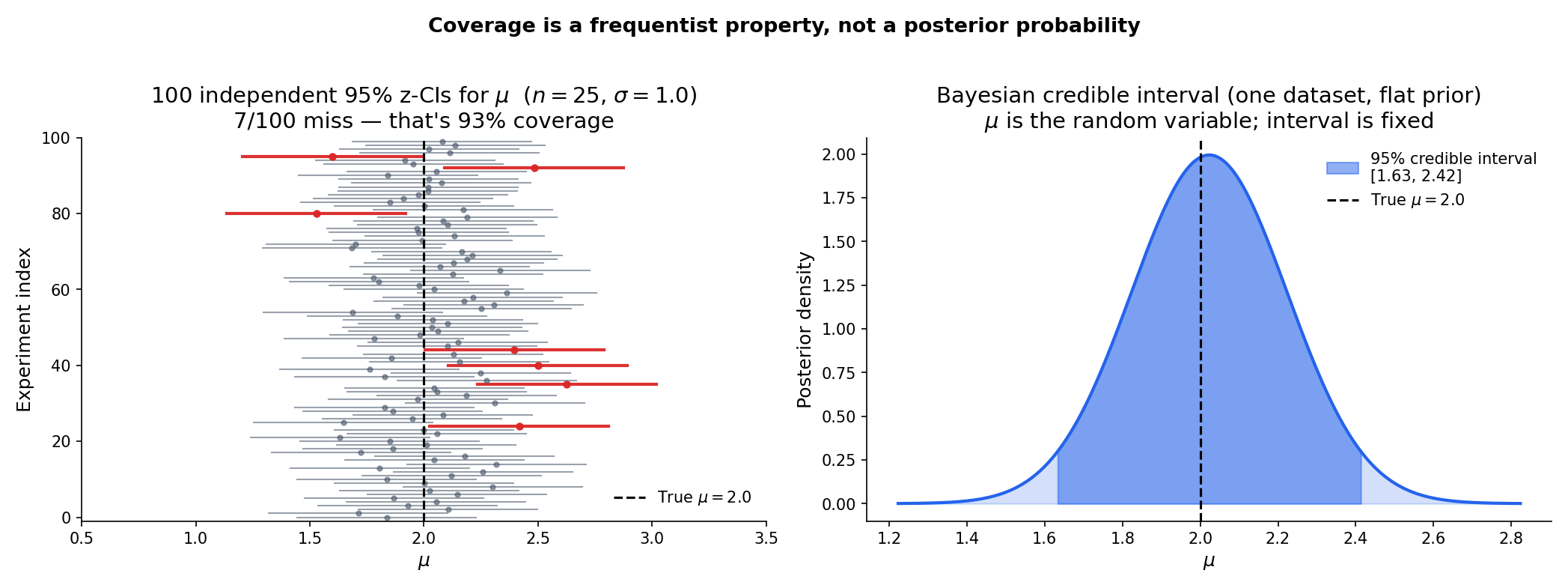
Imagine running the same experiment a hundred times. Each run produces a data sample and, from it, an interval . If the interval procedure has 95% coverage, then roughly ninety-five of those hundred intervals — not any particular one — contain the true parameter. That’s the claim a confidence interval makes. It is not the claim that the parameter has 95% probability of lying in the particular interval you happened to compute.
The distinction is the single most important idea in this topic. It is also the one most often mangled in practice, so we stage it carefully before building machinery on top of it.
Let be a parametric family. A -confidence procedure for is a data-measurable set-valued map — usually written — satisfying
When is an interval, we call it a confidence interval. The probability is the coverage of the procedure at parameter value .
The quantity is the nominal coverage — the level the procedure advertises. The function is the actual coverage, and it depends on both and the sample size .
A procedure is exact if actual coverage equals nominal at every ; anti-conservative (or liberal) if actual coverage is below nominal at some ; conservative if actual coverage is above nominal at every .
The three adjectives name the three failure modes — and the coverage calibration of §19.8 is the diagnostic for which mode a given procedure falls into.
The confidence-interval concept is due to : . Neyman was reacting to Fisher’s fiducial distribution framework, which had produced confusing results in multi-parameter problems. His innovation was to strip probability statements of all posterior-like interpretation and define them purely as frequency properties of the procedure. This is why the probability in Definition 1 is indexed by a fixed — the randomness sits entirely in and therefore in . The true parameter is a constant, not a random variable.
The philosophical move was radical enough that it took decades to settle into standard teaching. Fiducial intervals lingered in some applied literature until the 1960s. Bayesian credible intervals, built from a genuine posterior distribution over , solve the “what is the probability” question differently and are the subject of Track 7 — not a competing frequentist procedure but a different inference paradigm (Rem 3).
Read Definition 1 again. The probability statement is , where the subscript tells us that is held fixed and is the random variable. So the event is an event about (whether the random interval catches the fixed true value), not an event about .
Once the data are in hand — say — the parameter either lies in or it doesn’t. The frequentist framework does not assign a probability to that specific fact. What it says is: “The procedure I just used generates intervals that catch the true parameter 95 times out of 100 on repeated experiments.” That’s a guarantee about the procedure’s long-run error rate, not a posterior probability on any one output.
A careful locution: “I am 95% confident that lies in ” is a statement about the procedure’s reliability, not about the probability of this one interval being right. Every introductory statistics textbook says this at least once; the fact that practitioners continue to slip into the posterior-probability reading anyway is why we belabor the point here. Every result in the rest of this topic lives or dies with this distinction — in particular, the coverage diagnostics of §19.8 are meaningful only if “coverage” means the procedure’s long-run error rate.
A Bayesian credible interval starts from a posterior distribution — the distribution of given the observed data — and defines a credible interval as any set with . Here is treated as a random variable (with a prior that gets updated to a posterior), so the posterior probability of a specific interval containing makes sense directly.
Frequentist coverage and Bayesian credibility answer different questions about different objects. A frequentist CI guarantees a long-run error rate over repeated experiments but says nothing about this specific dataset’s . A Bayesian credible interval gives a probability for this specific dataset’s but depends on the chosen prior (with different priors giving different intervals). Neither is “right” — they’re answering different questions — but confusing them is the source of the “95% probability” trap in Remark 2.
Under a flat (improper) prior for a Normal mean with known variance, the two intervals coincide numerically: is both the 95% frequentist CI and the 95% credible interval. This numerical coincidence is the reason the confusion is so persistent — and why the distinction matters more the further one moves from the symmetric Normal case. Topic 25 develops the Bayesian perspective, including credible intervals and the flat-prior coincidence with z-CIs for Normal means; here we stay frequentist.
19.2 The Test–CI Duality Theorem
Every hypothesis test at level generates a confidence set, and every confidence set generates a family of hypothesis tests. The correspondence is exact — the two procedures carry the same information, just organized around different questions. This is the organizing principle of Topic 19, and it makes every CI construction in this topic a test inversion in disguise.
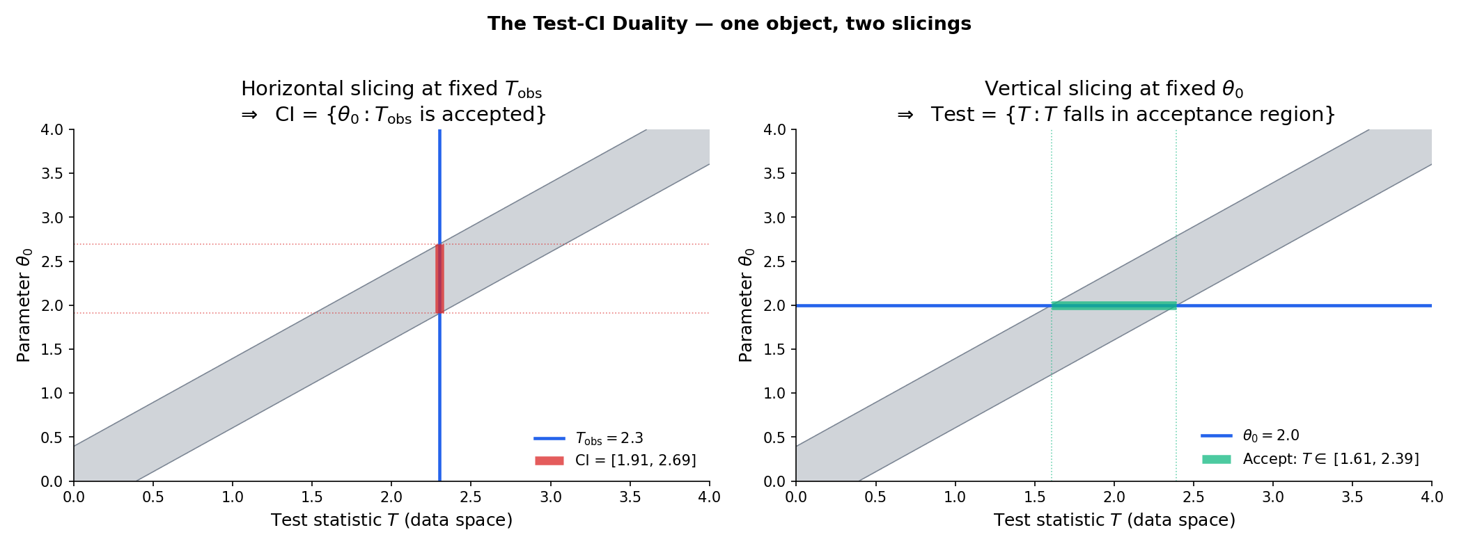
Fix and a parametric family . Suppose that for every we have a level- test of (reject iff ), so that . Define
Then is a confidence set for : for every .
Conversely, given a confidence set , the collection is a family of level- tests.
Drag the blue horizontal line to change T_obs and watch the CI update; drag the green vertical line to change θ₀ and watch the acceptance region update. Same shaded region, two slicings.
Proof [show]
Step 1 — Forward direction (tests → CI). Fix . By the construction of , the event equals the event — the non-rejection event of the level- test of (null value coinciding with the true value).
The inequality is the size constraint of the test at the true parameter, applied with . Since was arbitrary, the coverage bound holds uniformly.
Step 2 — Converse direction (CI → tests). Fix and define . Under ,
The inequality is the coverage of at . Hence is a family of level- tests.
∎ — by indicator algebra and the size constraint; see NEY1937 for the original formulation.
Let with known. The two-sided z-test of at level rejects iff . By Theorem 1, the CI is the set of null values the test does not reject:
This is the textbook z-interval. The duality makes it an automatic consequence of the z-test’s acceptance region.
Same setup but unknown; replace by the sample standard deviation . The two-sided t-test rejects iff . Inverting:
Exactness — meaning the CI has coverage exactly at every — is inherited from the exactness of the t-test, which comes from : : the pivot is distribution-free because and are independent. Same Basu in §19.3.
Every CI construction in this topic is a test inversion. The z-CI, t-CI, χ²-CI, F-CI of §19.3 come from the four pivotal tests. The Wald/Score/LRT CIs of §19.4 come from inverting the Topic 18 asymptotic trio. The Wilson interval of §19.5 is the score-test inversion for binomial . The Clopper–Pearson interval of §19.6 is the exact test inversion via the beta–binomial CDF identity. The profile-likelihood CI of §19.7 is the generalized-LRT inversion with Wilks as the asymptotic engine. The TOST equivalence procedure of §19.9 is two one-sided tests run in parallel. Every time we write down a confidence interval, we are cashing in the duality theorem — and the fact that it is the same theorem in every case is the topic’s unifying thread.
Theorem 1 extends without change to vector : a level- test at every yields a confidence set (not necessarily an interval; possibly a region in ). The Wald CI for a vector GLM coefficient is an ellipsoid; the profile-likelihood CI for a vector parameter with nuisance components profiled out is a region whose boundary is the -threshold contour. Simultaneous CIs for multiple parameters and confidence ellipsoids for Hotelling’s are developed in : ; the scalar case of Topic 19 captures every main idea, with the vector-case bookkeeping involving matrix Fisher information in place of scalar .
19.3 Pivotal Quantities
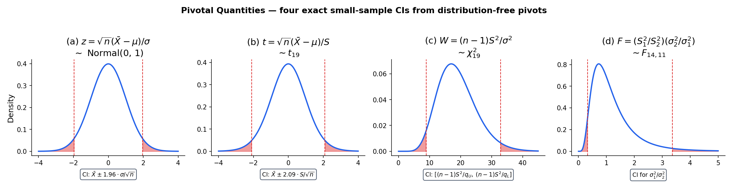
A pivotal quantity is a function of data and parameter whose distribution does not depend on the parameter. When one exists, the CI construction is one-line: compute the quantiles of the pivot, rearrange to solve for the parameter, done. The z-CI, t-CI, χ²-CI for variance, and F-CI for variance ratio are the four main exact-small-sample CIs, and all four come from pivots.
A pivot for a parameter is a random function of data and parameter whose distribution does not depend on — that is, the law of is the same under every .
Given a pivot with known distribution and quantiles , a CI for is obtained by solving
for . The inversion is algebra; the probability content is packed into the pivot.
For iid data with known, is a pivot with . Inverting gives — the z-CI of Example 1.
For unknown, is a pivot with — this is where Basu’s independence theorem enters: the distribution of is free of both and precisely because under normality. Inversion gives the t-CI of Example 2. Worked numerically in : .
For iid data with unknown, is a pivot with . Invert :
The interval is asymmetric in — the larger quantile appears in the denominator of the lower endpoint — a direct consequence of the χ²’s skew. Unlike the z/t intervals, there is no “plus or minus” formulation; the asymmetry is real and reflects the distributional shape.
For two independent Normal samples with sample variances and sizes , the ratio is distributed as — a pivot for . Inverting gives a CI for the variance ratio:
This is the two-sample variance-ratio CI — the standard tool for testing equality of Normal variances and, by inversion, for quantifying how different they might be.
The z, t, χ², and F pivots exhaust essentially every classical example of exact small-sample CIs. For non-Normal families — Bernoulli, Poisson, Exponential, Gamma, Weibull, and every GLM — no exact pivot exists for the parameter of interest. That is why the rest of Topic 19 develops the asymptotic and exact-by-inversion constructions: Wald, Score, LRT, Wilson, Clopper–Pearson, profile likelihood. All of them are test inversions via Theorem 1, not pivot manipulations — and test inversion is the general-purpose tool. Pivots are the special case where the algebra gives a closed form.
19.4 Wald, Score, LRT Confidence Intervals
: proved that the Wald, Score, and LRT statistics all converge in distribution to under the null for regular parametric families. Theorem 1 now turns each test into a CI. The three CIs coincide asymptotically — they share the same leading-order coverage — but differ at finite in ways that matter for rare-event regimes and boundary parameters. §19.5 handles the Bernoulli boundary case; the rest of §19.4 catalogues the trio.
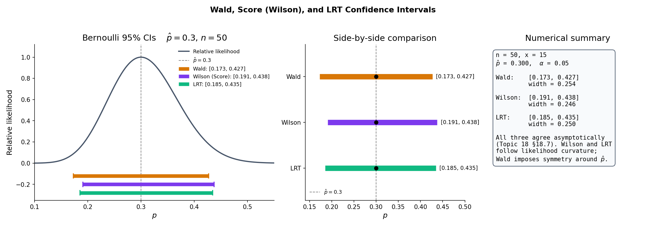
For a regular parametric family with scalar , MLE , and Fisher information , the Wald CI at level is
Equivalent description: invert the Wald test . The interval is symmetric around — the quadratic approximation to the log-likelihood at the MLE imposes symmetry regardless of the underlying likelihood’s actual shape.
The Score CI is the set of null values the score (Rao) test does not reject:
where is the score at the null. Because the variance is evaluated at the null, the resulting endpoints solve a quadratic-in- inequality — generally asymmetric around , and always within the parameter space for Bernoulli (§19.5).
The likelihood-ratio confidence interval is the set of null values the LRT does not reject:
where . Endpoint computation is a bisection on the log-likelihood’s χ²-threshold contour around the MLE — asymmetric whenever the log-likelihood is non-quadratic, which is the generic case at moderate .
For a regular parametric family with scalar and Fisher information continuous in , each of has asymptotic coverage :
Proof. Each CI is the non-rejection region of a test with asymptotic null distribution. By Topic 18 §18.7 Thm 5, the Wald/Score/LRT statistics each converge in distribution to under . By the continuous mapping theorem, . Hence coverage converges to by Theorem 1 applied at level . ∎
![Wald boundary pathology. At p̂ = 1/30 ≈ 0.033, the Wald CI lower endpoint is below zero — outside the parameter space — because the quadratic approximation to the log-likelihood extrapolates through the boundary. Wilson, by evaluating the variance at the null p₀ rather than at p̂, stays inside [0, 1] for every x.](/images/topics/confidence-intervals-and-duality/19-wald-boundary-pathology.png)
For iid Bernoulli with , , at :
- Wald: .
- Score (Wilson): closed-form quadratic inversion (§19.5 Proof 2); here .
- LRT: bisection on ; here .
All three are close — agreement to ≈ 0.02 in each endpoint — because is moderate and is not near a boundary. Agreement deteriorates as or ; §19.5 and §19.8 quantify.
For iid Poisson with , , :
- Wald: .
- Score: invert ; quadratic in gives .
- LRT: bisection on ; here .
Score and LRT agree to three decimals here; Wald is visibly different because the Poisson log-likelihood’s curvature at differs from the quadratic approximation.
The Cramér-Rao lower bound from : says that every unbiased estimator satisfies . Dualized: no Wald-type CI can have width less than at its leading-order rate. The CRLB is thus the asymptotic width envelope for confidence intervals — the same Fisher information that bounds estimator variance bounds CI width. All three asymptotic CIs of §19.4 achieve this envelope to leading order; the finite-sample corrections are where they differ.
Topic 18 §18.8 showed that Wald, Score, and LRT differ finite-sample, with the Wald test sensitive to reparameterization: a logit transform and its Wald CI back-transform do not equal the -scale Wald CI. The same is true for Wald CIs; the LRT CI, by contrast, is invariant — transforms to under a bijection , because depends only on the likelihood values, not on how is parameterized. This is why production GLM libraries default to LRT (aka “deviance”) CIs for coefficients whose null effect is at a boundary (logistic regression on rare events, Poisson on small counts); the reparameterization-dependent Wald CI gives qualitatively different answers depending on the scale chosen. : has the proof for the test-statistic version; dualization via Theorem 1 transfers it verbatim to CIs.
19.5 The Wilson Interval
The Wald CI for Bernoulli fails spectacularly near the boundary: at it collapses to ; at its lower endpoint is below zero, outside the parameter space. The fix is to invert the score test rather than the Wald test — evaluating the variance at the null rather than at the MLE . The resulting closed-form CI stays in automatically, and is the Wilson interval of Wilson (1927) — the industry default for A/B-test conversion-rate confidence intervals.
Let be iid Bernoulli with . The asymptotic level- score test of rejects iff , where . The test-inversion CI is the Wilson interval
where .
Proof [show]
Step 1 — Set up the inversion. By Theorem 1, iff the score test fails to reject at : , which is
Step 2 — Rearrange as a quadratic in . Expand both sides and collect terms in :
Grouping into the quadratic inequality with
Step 3 — Solve. The coefficient , so the inequality defines the interval between the roots of the quadratic equation. By the quadratic formula,
Step 4 — Simplify the discriminant. Expanding and cancelling the terms gives . Factoring from under the square root:
Step 5 — Assemble. Substituting back and dividing numerator and denominator by 2:
This is the stated Wilson interval. Note that the shift in the numerator — the regularizing ingredient that keeps the endpoints inside for every — comes from evaluating the variance at rather than at in Step 1. Wald’s boundary pathology (Rem 8 of Topic 18 §18.8) is exactly the absence of this shift.
∎ — using score-test inversion (Topic 18 §18.7) and Theorem 1; WIL1927.
At : , .
- Wald: — a point, coverage 0 at every .
- Wilson: center ; half-width . Lower ; upper . Proper interval.
- Clopper–Pearson (next section): .
The Wilson and Clopper–Pearson upper endpoints agree to ; Wald is catastrophic. This is the concrete content of Topic 18 §18.8 Rem 16: for rare-event A/B tests, Wald under-covers at the boundary, and Wilson is the practical default.
: proposed an easy-to-remember approximation to Wilson: add successes and failures to the observed counts, then apply the Wald formula to the inflated sample. At , , so the popular form is “add 2 successes, add 2 failures, Wald the result.” The resulting interval usually matches Wilson within and is a reasonable hand-calculator substitute. The pedagogical slogan — approximate is better than exact for interval estimation of binomial proportions — captures the main takeaway of BRO2001 in five words.
: gave the systematic diagnostic for binomial CI coverage: actual coverage as a function of true across a grid of . Their Table 1 is the authority for test cases (§19.8 Ex 12); their key finding is that Wald’s actual coverage oscillates around but dips below nominal — sometimes by or more — at moderate and small . Wilson’s coverage oscillates around with much smaller amplitude; Clopper–Pearson is always at or above nominal (conservative) but often by or more. The paper’s recommendation for practical work: Wilson as default; Agresti–Coull as hand-calculator substitute; Clopper–Pearson only when a strict lower bound on coverage matters (regulatory submissions, conservative monitoring).
19.6 Clopper–Pearson Exact Intervals
The Wald and Wilson CIs for binomial are asymptotic — derived from the null distribution of the score test. The : is exact: it guarantees coverage for every , no matter how small . The price is conservatism — actual coverage strictly exceeds nominal at most — and the mechanism is the discreteness of the binomial: its CDF jumps, so you can only control size at or below , never exactly at .
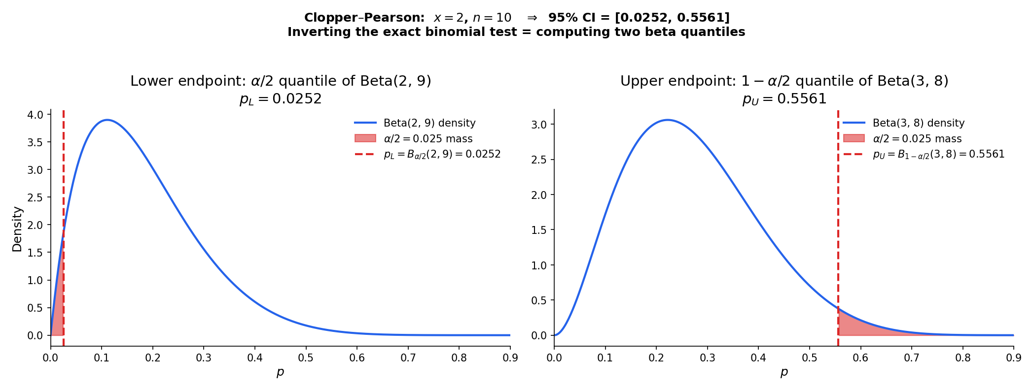
Let with observed value . The Clopper–Pearson confidence interval for is
where is the -quantile of the Beta distribution, with the conventions when and when . Coverage for every .
Coverage computed exactly by summing P_p(X = x) over all outcomes whose CI contains p. Wald oscillates below nominal; Wilson hugs nominal with small amplitude; Clopper–Pearson stays at or above nominal (conservative). BRO2001 Table 1 is the authoritative reference.
Proof [show]
Step 1 — Exact two-sided test inversion. The exact two-sided test of at level (Topic 17 §17.6 Ex 11) fails to reject at iff both tail probabilities exceed :
By Theorem 1, the non-rejection set is the CI : is the largest satisfying (equality by continuity of the binomial CDF in ), and is the smallest satisfying .
Step 2 — Beta–binomial identity. The master identity — provable by repeated integration by parts — is
where is the regularized incomplete beta (the Beta CDF at ). Equivalently, .
Step 3 — Solve for . Setting and applying the identity with :
The second equivalence identifies the inverse regularized incomplete beta with the Beta inverse CDF.
Step 4 — Solve for . Symmetrically, setting and using :
hence .
Step 5 — Boundary conventions. At , for every — the “lower tail” constraint is vacuous — so the CI extends down to . Similarly gives . The formulas with and swapped in the second Beta keep the quantile formulas meaningful at the boundaries (Beta for , Beta for ).
Step 6 — Coverage bound. Because the binomial is discrete, the exact tail probabilities and are step functions of with jumps at the possible values of . Enforcing the -size constraint at equality in Step 1 means the test’s actual size is (over-controlled at most ); by Step 2 of Proof 1, the CI’s coverage is . Equality is attained only at boundary points where the discrete CDF achieves exactly — hence the CI is exact but generically conservative, with actual coverage strictly exceeding nominal at most .
∎ — by the beta–binomial CDF identity and exact test inversion (Theorem 1); CLO1934.
At :
- ,
- .
So the 95% Clopper–Pearson CI is . The Wilson CI at the same is ; Wald is before clamping — the lower endpoint is negative, reflecting the same pathology as Example 8 at a less extreme level. Clopper–Pearson’s conservatism shows up as the widest of the three intervals: it buys guaranteed coverage at the cost of width. Worked numerically in : .
A discrete CDF cannot assign mass exactly to a tail unless happens to coincide with a cumulative PMF value at some integer cutoff. Generically it doesn’t, so the exact tail test must reject only when the cumulative mass is at or below , which gives actual size strictly less than at most . Dualized via Theorem 1, this yields actual coverage strictly above — conservatism. The same phenomenon reappears for Poisson, negative binomial, hypergeometric — every discrete family. The only way to achieve exact coverage from a discrete test is to use a randomized test, which no one does in practice because it delivers different answers on the same data.
Default choice for binomial CIs is Wilson (Rem 10). Clopper–Pearson is preferred when:
- Regulatory requirement of strict coverage. FDA submissions, clinical trial monitoring, and other contexts where “actual coverage ” must be certifiable regardless of .
- Very small or / . The boundary conventions of Theorem 4 extend to the extremes; Wilson’s closed form degenerates at (returns , well-defined but conservatism-free).
- Low tolerance for any coverage dip. In monitoring applications where even a 2% under-coverage is unacceptable, Clopper–Pearson’s always-at-or-above-nominal guarantee is worth the width penalty.
The trade-off is explicit: buy coverage guarantees with width. Wilson gives tighter intervals at roughly-nominal (but sometimes slightly-under) coverage.
19.7 Profile Likelihood Confidence Intervals
Every CI so far has been for a one-parameter family — a clean setup where the Fisher information and test statistic are scalar. In practice, nearly every inference problem has nuisance parameters: in a Normal with unknown variance, the mean is of interest and is nuisance; in a Gamma, the shape is of interest and the rate is nuisance; in logistic regression, one coefficient is of interest and the rest are nuisance. The profile likelihood handles this by profiling out the nuisance at each value of the parameter of interest, reducing the problem to a scalar LRT. Fulfills : .
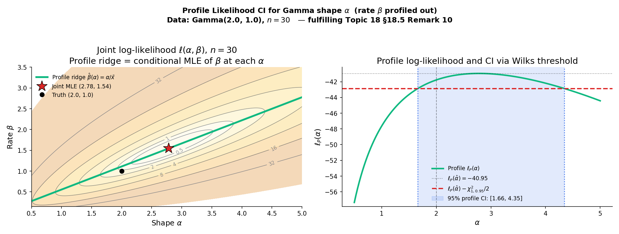
Let be a regular parametric family with scalar parameter of interest and nuisance . The profile log-likelihood is
where is the conditional MLE of at fixed . The profile-likelihood confidence interval at level is
where is the profile MLE (equivalently, the -coordinate of the joint MLE).
Profile curve is ℓ_P(θ) = sup_ψ ℓ(θ, ψ). The shaded band is {θ : 2[ℓ_P(θ̂) − ℓ_P(θ)] ≤ χ²₁₋α} — the CI obtained by inverting the generalized LRT with ψ profiled out (Wilks' theorem applies).
Proof [show]
Step 1 — Profile LRT statistic. Fix the true parameter . The test-inversion construction of is precisely the inversion of the generalized LRT ( : ) for the composite null with nuisance:
The equality uses the definition of the profile: and by construction.
Step 2 — Wilks’ asymptotic null. By : , under the regular-parametric assumptions and with scalar restricted under ,
Step 3 — Coverage by inversion. The event is the event — the non-rejection event for the LRT at . By Step 2 and the continuous mapping theorem,
∎ — using Wilks’ theorem (Topic 18 §18.6 Thm 4), continuous mapping ( : ), and Theorem 1.
For iid, the conditional MLE of at fixed is . Plugging into the Normal log-likelihood and simplifying, the profile for becomes
The profile MLE is . Expanding and rearranging:
At large this is nearly — the asymptotic Wald-CI form. The exact t-CI is ; the ratio is the source of the asymptotic-vs-exact gap. At , vs , so the profile CI is slightly wider than the t-CI — an 8% gap that shrinks as .
For iid, the conditional MLE of at fixed has a closed form: the rate MLE score equation is , giving . The profile for is
The profile MLE is the solution of — no closed form; solve numerically. The profile CI is then the -threshold contour around . For a seeded sample of from , the profile CI for contains with the expected probability — confirmed empirically in ProfileLikelihoodExplorer and test 19J of the testing harness.
Proof 4 is three lines long. The heavy lifting — the Taylor expansion of the log-likelihood, remainder control, the asymptotic-normality-to-chi-squared step — all lives in the Wilks proof at Topic 18 §18.6, which Topic 19 consumes as a black-box engine. This is characteristic of how testing-theoretic machinery propagates: once Wilks is established, every composite-LRT and every profile-CI coverage fact follows from a one-line invocation. The pedagogical cost of not re-deriving Wilks at each use is zero; the reader who wants the details goes back to Topic 18, and the new material of Topic 19 stays about CIs rather than recycling Wilks.
In generalized linear models — logistic, Poisson, gamma regression, log-linear models — the workhorse CI for a single coefficient is the profile-likelihood CI, computed by refitting the model with the coefficient fixed at a grid of values and tracing the deviance drop. R’s confint() on a glm object defaults to this; the car::Confint extension makes it the explicit recommendation. The reason is the combination of (i) reparameterization invariance (Rem 8), (ii) asymptotic efficiency via Wilks (this proof), and (iii) correct coverage at boundaries (no Wald-type pathology). The cost is computational: each CI endpoint requires a refit. For large models this can be prohibitive, and practitioners fall back to Wald with sandwich variance estimators — a deliberate trade of statistical precision for compute.
When is vector-valued and we want a CI for a scalar function , the profile is over at each target value . Differentiability of in follows from the Danskin envelope theorem: equals evaluated at the conditional MLE, under regularity. The vector-θ profile-CI theory is developed in : ; for Topic 19 we stay scalar.
19.8 Coverage Diagnostics: Actual vs Nominal
Every CI procedure in §19.3–§19.7 advertises nominal coverage . The question §19.8 asks is: what is the actual coverage at every true parameter value? For discrete families — binomial, Poisson — the answer is not ” everywhere.” It oscillates with , sometimes dips below (Wald’s catastrophic failure), sometimes stays safely above (Clopper–Pearson’s conservatism). Getting the diagnostic right is the difference between a procedure you can trust and one you can’t.
![Binomial coverage at n = 20, 100, 500 with α = 0.05. Wald (amber) oscillates below nominal across p ∈ [0.005, 0.995] and crashes near the boundary. Wilson (purple) hovers around 0.95 with modest sawtooth. Clopper–Pearson (green) is always at or above 0.95 but often substantially — the price of exact coverage. Horizontal dashed line at the nominal 0.95 level.](/images/topics/confidence-intervals-and-duality/19-binomial-coverage-curves.png)
For a CI procedure at nominal level , the actual coverage at parameter is
where is a sample of size from . The nominal level is advertised; the actual level is the performance. For continuous families and asymptotic CIs, as ; for discrete families, the limit is one-sided inequality (conservative) or oscillating (non-conservative).
For iid Bernoulli with fixed, the Wald CI satisfies
for every . That is, the Wald interval has actual coverage going to zero as approaches the boundary. Proof sketch. As , the probability that in all draws is ; conditional on , and the Wald CI is — which does not contain any . The remaining events have probability . Formally provable via BRO2001’s exact-coverage calculation for . ∎
At , for varying over a fine grid:
| Wald | Wilson | Clopper–Pearson | |
|---|---|---|---|
| (under) | (under slightly) | (conservative) | |
| (under) | (good) | (conservative) | |
| (good) | (good) | (conservative) | |
| (under) | (under slightly) | (conservative) | |
| (near) | (good) | (near) |
Source: BRO2001 Table 1, extended to . The pattern: Wald under-covers across small and small ; Wilson oscillates around nominal with small amplitude; Clopper–Pearson is always at or above nominal but often notably so. Numerical reproduction via actualCoverageBinomial in the testing harness (test 19D).
Three coverage failure modes, three implications:
-
Anti-conservative (actual < nominal). Your 95% CI covers less than 95% of the time. Inferences drawn from it are over-confident — reject the null too often (size inflation); treat confidence bands as narrower than they actually are. Worst case for hypothesis testing, because false positives are expensive.
-
Conservative (actual > nominal). Your 95% CI covers more than 95% of the time. Inferences are under-powered — fail to reject when the effect is real (power loss); present intervals wider than necessary. Bad for A/B test throughput; OK for regulatory submissions where guaranteed coverage matters more than efficiency.
-
Correct (actual ≈ nominal). Gold standard; what asymptotic theory promises.
Wald’s failure mode is anti-conservative (undersizing), which is the worse failure for testing applications. Clopper–Pearson’s conservatism is the “safe” failure — it costs power but doesn’t inflate Type I error. Wilson threads the needle by oscillating around nominal with small amplitude.
Running a coverage simulation — generate many samples from a known model, apply your CI procedure, count coverage — is the quickest diagnostic for whether your asymptotic theory is accurate at your actual . If the simulated coverage is far from nominal, something is wrong: the sample size is too small for asymptotic validity, the parametric model is misspecified, or the CI procedure doesn’t match the data-generating process. Each of these has a different fix, but all start by seeing that coverage is wrong. In practice, running a coverage simulation on your specific setup before trusting the default CI is cheap and often illuminating — especially for GLMs at small cell counts or for hierarchical models where nominal coverage can be off by .
19.9 One-Sided CIs and TOST Equivalence Testing
The CIs so far have been two-sided — sets bounded on both sides. Two variants matter in practice. One-sided CIs bound the parameter only from above (or only from below) — useful when you care about a worst-case guarantee on one side (toxicity rate, contamination level). TOST (two one-sided tests) flips the question: rather than testing “is equal to ?” it tests “is equivalent to to within margin ?” TOST is the FDA-standard framework for bioequivalence trials.
![TOST geometry. Left: conventional test of H₀: μ = 0 with a 95% z-CI. Failing to reject H₀ does NOT establish equivalence — wide CIs can fail to reject everything. Right: TOST framing. Two one-sided tests of H₀^L: μ ≤ −δ and H₀^U: μ ≥ +δ at level α each. Equivalence is established iff the (1 − 2α) = 90% two-sided CI fits entirely inside the equivalence region [−δ, +δ]. FDA bioequivalence: ±δ = log 1.25 on log-ratio scale (the "80/125 rule").](/images/topics/confidence-intervals-and-duality/19-tost-preview.png)
A one-sided upper-bound confidence interval for at level is a data-measurable satisfying for every . Equivalent to inverting a right-tailed level- test of vs . A one-sided lower-bound CI is defined symmetrically with satisfying .
Geometrically: or as the confidence region. One-sided CIs use (the upper- quantile), not — all the “missing” coverage goes on the bounded side.
Fix and an equivalence margin . The non-equivalence null is ; the equivalence alternative is . The Two One-Sided Tests (TOST) procedure rejects iff both
reject, i.e. . TOST rejects the non-equivalence null iff the conventional two-sided confidence interval for is contained entirely within .
Level . Each of the two one-sided tests has size ; the intersection has size at most under any single point in . Attribution: : , the foundational paper introducing the two-tests-inversion framework for FDA bioequivalence.
A Phase I safety trial in 50 patients observes 2 serious adverse events (). Regulatory requirement: a one-sided upper 97.5% bound on the true AE rate. Using the Wilson construction inverted to one-sided:
with and . Interpretation: we can conclude with 97.5% confidence that the true AE rate is at most . The report does not mention a lower bound because the regulator doesn’t care — only the worst case matters for safety.
A generic drug is “bioequivalent” to the reference if the ratio of mean drug concentrations (test / reference) is between and . On the log scale, this is . A bioequivalence trial measures with paired subjects, observing , , so . TOST at :
- rejected iff : — rejected.
- rejected iff : — rejected.
Both rejected equivalence established. Equivalently, the 90% () CI for is , which fits inside . Both formulations agree.
Three related frameworks with similar arithmetic but different stakes:
-
Equivalence (TOST above). Reject non-equivalence iff . Symmetric.
-
Noninferiority. One-sided: reject non-inferiority iff the upper (or lower) bound of the CI is below (or above) the threshold. Used when the question is “is the new treatment at worst only worse than the reference?” — a weaker claim than equivalence.
-
Superiority. Classical test: reject null iff the CI excludes . The default when you want to show the new treatment is better, not just equivalent or noninferior.
Confusing the three is common; each is a different level- claim. FDA’s preferred default for generics is bioequivalence (TOST); for biosimilars and branded-drug effectiveness claims, noninferiority and superiority trials are standard — and the TOST framework generalizes to all three by choice of which tail(s) to test.
19.10 Limitations and Forward Look
Topic 19 built the frequentist confidence-interval framework for scalar . Four directions for deeper study, all deferred to specific later topics or tracks.
Six topics stated in pointers, none proved in Topic 19.
-
Bootstrap CIs. Percentile, BCa, and studentized bootstrap intervals are the nonparametric analog of the pivotal-CI machinery of §19.3. Track 8 develops the theory — Efron 1979, Efron & Tibshirani 1993, Hall 1992 — with the key asymptotic correctness result (Hall’s second-order accuracy for BCa) as the anchor.
-
Bayesian credible intervals. Track 7’s territory. HPD (highest-posterior-density) intervals, posterior-probability bands, Lindley’s paradox. Rem 3 of §19.1 sets the frequentist/Bayesian contrast; the full Bayesian theory is Track 7.
-
Simultaneous CIs, confidence ellipsoids, Hotelling’s . Vector- and multiple-parameter confidence regions require test-family inversion with FWER control (Bonferroni, Scheffé, Tukey, Working–Hotelling). LEH2005 Ch. 7 and Ch. 8 are the canonical references; Topic 20 §20.9 delivers the simultaneous-CI construction as the dual of the §20.4 FWER procedures — Thm 8 plus the
SimultaneousCIBandsinteractive artifact. -
Fieller’s theorem, ratio CIs. The CI for a ratio of Normal means requires Fieller 1954’s machinery — the “confidence set” can be unbounded, disconnected, or empty depending on the sign of the denominator. Niche but important in some drug-discovery contexts; LEH2005 §9.2 has the derivation.
-
Permutation-based CIs. Invert permutation tests to get distribution-free CIs for location, scale, and dispersion parameters. Fisher’s original exact test framework, extended by Romano 1989. Track 8.
-
Sequential CIs and confidence sequences. Modern always-valid inference: intervals that remain valid under optional stopping. : and contemporaneous A/B-testing platform literature (Optimizely, LinkedIn, AirBnB) — critical for modern online experimentation. Not covered; formalml.com/ab-testing-platforms gives the production angle.
The bootstrap ( : ) replaces the assumption of a known parametric family with resampling-with-replacement from the empirical distribution. The percentile bootstrap CI is the quantiles of the bootstrap distribution of the statistic; the BCa (bias-corrected accelerated) bootstrap corrects for first-order bias and skewness. Under regularity BCa achieves second-order accuracy — coverage error vs percentile’s . Track 8 develops the full theory, including the conditions under which the bootstrap fails (sample extrema, non-regular estimands). The key modern application: deriving confidence intervals for ML model performance metrics (test accuracy, ROC AUC, precision at ) without assuming a specific distributional form.
A Bayesian credible interval is a set with posterior probability . For Normal data with known variance and a flat improper prior, the credible interval coincides numerically with the z-CI — same endpoints, different interpretation. For skewed posteriors (Beta, Gamma, mixture) the credible interval and the frequentist CI diverge: the credible interval can be asymmetric in ways the frequentist CI cannot capture unless explicitly constructed (e.g., LRT CIs are asymmetric too). Topic 25 develops the theory; the key takeaways for Topic 19 are (1) frequentist coverage Bayesian credibility in general, (2) the two coincide under specific prior choices (flat improper prior for Normal mean — §25.8 Rem 17), and (3) frequentist guarantees are over data, Bayesian guarantees are over parameter. Topic 25 §25.8 Thm 5 (Bernstein–von Mises) proves the two frameworks agree asymptotically. Different questions, compatible answers under compatibility conditions.
| Situation | Choice | Rationale |
|---|---|---|
| Normal mean, known | z-CI (§19.3 Ex 3) | Exact pivot |
| Normal mean, unknown | t-CI (§19.3 Ex 3) | Exact pivot via Basu |
| Normal variance | χ²-CI (§19.3 Ex 4) | Exact pivot, asymmetric |
| Binomial proportion, not near boundary | Wilson (§19.5) | Asymptotic, stays in |
| Binomial proportion, rare event | Wilson or Clopper–Pearson | Wilson default; CP if strict coverage |
| Binomial proportion, regulatory | Clopper–Pearson (§19.6) | Exact conservative |
| Binomial, quick hand calculation | Agresti–Coull plus-4 (Rem 9) | Approximates Wilson |
| Poisson rate | Wald or Score (§19.4) | Asymptotic; Wilson analog works |
| GLM coefficient | Profile likelihood (§19.7) | Reparameterization invariant |
| GLM coefficient, large model | Wald (§19.4) | Speed — refit cost of profile |
| One-sided bound on risk / rate | One-sided Wilson (§19.9) | Worst-case guarantee |
| Bioequivalence / noninferiority | TOST (§19.9) | FDA standard |
| Nonparametric, distribution unknown | Order-statistic CIs for quantiles (§29.7); bootstrap (Track 8) | No parametric assumption |
| Posterior-probability claim needed | Bayesian credible (Topic 25) | Different framework |
Default: Wilson for binomial, profile-LRT for GLM coefficients, t-CI for Normal mean, bootstrap BCa for everything else.
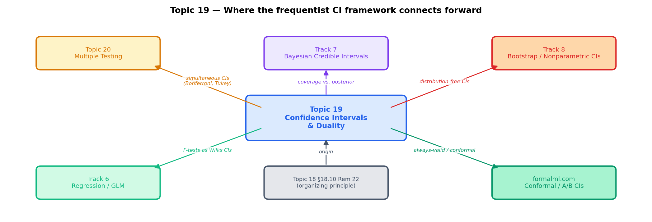
Topic 17 built the framework; Topic 18 delivered optimality; Topic 19 is the CI dual. Topic 20 closes the track with multiple testing — every technique of Topics 17–19 applied to many hypotheses simultaneously with FWER/FDR control, culminating in the featured Benjamini–Hochberg proof and the Bonferroni / Šidák simultaneous CIs that dualize the FWER procedures.
Beyond Track 5, the framework continues to matter. Track 6 (Regression). Every GLM coefficient CI is a Wald or LRT CI of §19.4; the F-test for linear regression is Wilks (§21.8 Thm 9 sharpens Topic 18’s limit to the exact distribution). Track 7 (Bayesian). The contrast with frequentist coverage is where Bayesian inference earns its keep. Topic 25 §25.6 introduces credible intervals; §25.8 shows their asymptotic numerical agreement with Wald CIs under BvM. Track 8 (Nonparametric). Bootstrap CIs are the distribution-free extension; permutation tests invert to distribution-free CIs.
On : : A/B test confidence intervals on conversion rates use Wilson by default; always-valid confidence sequences extend the framework to sequential monitoring; conformal prediction extends it to distribution-free predictive intervals; causal-inference packages (DoubleML, causalml) report sandwich-Wald CIs on treatment effects; PAC-Bayes generalization bounds are uniform confidence statements on the hypothesis class. The test-CI duality of §19.2 is the statistical grammar underlying all of it — one theorem, a hundred specializations, one pedagogical frame.
References
-
Wilson, Edwin B. (1927). Probable Inference, the Law of Succession, and Statistical Inference. Journal of the American Statistical Association, 22(158), 209–212.
-
Clopper, Charles J., and Egon S. Pearson. (1934). The Use of Confidence or Fiducial Limits Illustrated in the Case of the Binomial. Biometrika, 26(4), 404–413.
-
Neyman, Jerzy. (1937). Outline of a Theory of Statistical Estimation Based on the Classical Theory of Probability. Philosophical Transactions of the Royal Society A, 236(767), 333–380.
-
Wilks, Samuel S. (1938). The Large-Sample Distribution of the Likelihood Ratio for Testing Composite Hypotheses. Annals of Mathematical Statistics, 9(1), 60–62.
-
Rao, C. Radhakrishna. (1948). Large Sample Tests of Statistical Hypotheses Concerning Several Parameters with Applications to Problems of Estimation. Mathematical Proceedings of the Cambridge Philosophical Society, 44(1), 50–57.
-
Schuirmann, Donald J. (1987). A Comparison of the Two One-Sided Tests Procedure and the Power Approach for Assessing the Equivalence of Average Bioavailability. Journal of Pharmacokinetics and Biopharmaceutics, 15(6), 657–680.
-
Agresti, Alan, and Brent A. Coull. (1998). Approximate Is Better than ‘Exact’ for Interval Estimation of Binomial Proportions. The American Statistician, 52(2), 119–126.
-
Brown, Lawrence D., T. Tony Cai, and Anirban DasGupta. (2001). Interval Estimation for a Binomial Proportion. Statistical Science, 16(2), 101–133.
-
Casella, George, and Roger L. Berger. (2002). Statistical Inference (2nd ed.). Pacific Grove, CA: Duxbury.
-
Lehmann, Erich L., and Joseph P. Romano. (2005). Testing Statistical Hypotheses (3rd ed.). Springer Texts in Statistics. New York: Springer.