intermediate 60 min read · April 22, 2026

Hierarchical & Empirical Bayes

Topic 28 closes Track 7 by bending the tools of Topics 25–27 onto structures where group-level parameters share a common distribution and the prior itself has a prior. Eight schools as the spine example. Three full proofs — Stein's paradox via Stein's identity (featured), the partial-pooling shrinkage formula in the Normal–Normal hierarchy, and volume preservation + funnel decoupling for the non-centered reparameterization. Empirical Bayes as the boundary case. Linear mixed-effects. HMC diagnostics. The forward-map to formalml closes the track.

formalCalculus: multivariable integration formalCalculus: gradient and directional derivatives formalML: sparse bayesian priors formalML: variational inference formalML: bayesian neural networks formalML: bayesian nonparametrics formalML: meta learning formalML: mixed effects

28.1 Three ways to pool, one dataset

Eight schools each ran a short-term coaching program for the SAT-verbal section. Each school estimates its own treatment effect $y_k$ with a standard error $\sigma_k$ that reflects its sample size. The data, from Rubin’s 1981 analysis (RUB1981, reproduced in GEL2013 §5.5):

School	A	B	C	D	E	F	G	H
$y_k$ (effect estimate, SAT-V points)	28	8	−3	7	−1	1	18	12
$\sigma_k$ (standard error)	15	10	16	11	9	11	10	18

The effects are plausibly between $-20$ and $+30$ and the standard errors are large — 28 and $-3$ may just be noise around a common truth, or they may be real differences between schools. The question is how to estimate each school’s effect given all the data.

Three answers sit at the extremes and the middle.

No pooling. Treat each school as its own problem: $\hat\theta_k = y_k$ . Honest about between-school differences, but hostage to each $\sigma_k$ . School A’s 28-point estimate carries a $\pm 15$ -point standard error — we shouldn’t read too much into it.
Complete pooling. Treat all schools as one problem: $\hat\theta_k = \hat\mu$ for every $k$ , where $\hat\mu = \sum_k (y_k / \sigma_k^2) / \sum_k (1/\sigma_k^2)$ is the precision-weighted grand mean ( $\approx 7.69$ here). Huge precision gain, but tosses out any real differences.
Partial pooling. Assume the $\theta_k$ are drawn from a common distribution $\mathcal{N}(\mu, \tau^2)$ . Each school’s posterior mean becomes a precision-weighted compromise: $(1 - B_k) y_k + B_k \hat\mu$ with $B_k = \sigma_k^2 / (\sigma_k^2 + \tau^2)$ . Schools with small $\sigma_k$ stay close to $y_k$ ; schools with large $\sigma_k$ drift toward $\hat\mu$ . Both the between-school variance $\tau^2$ and the group means $\theta_k$ are learned from the same data.

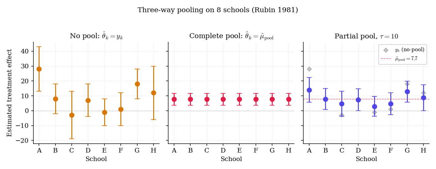
Figure 1. The three pooling regimes on 8-schools. Partial pooling is the middle panel — each school’s posterior mean is a weighted average of its raw estimate and the grand mean, with weights determined by the relative size of $\sigma_k^2$ (noise in $y_k$ ) and $\tau^2$ (spread across schools).

Topic 28 is the story of partial pooling. Six intertwined threads run through the next ten sections:

The hierarchical model as a two-level generative process (§28.2).
Full-Bayes inference via Gibbs + HMC, with §26.8 Rem 23’s 8-schools funnel (§28.4).
Stein’s paradox (§28.5): even when the group means are unrelated in truth, shrinkage toward any common target strictly dominates the MLE under squared-error loss in $d \geq 3$ dimensions. The pedagogical summit of Track 7.
Closed-form partial pooling in the Normal–Normal hierarchy (§28.6), with the shrinkage factor $B_k$ proved.
Empirical Bayes (§28.7): $\mu$ and $\tau^2$ learned from the data via Type-II MLE; the 8-schools boundary case $\hat\tau^2 \approx 0$ motivates full-Bayes over EB.
Non-centered reparameterization (§28.9 Thm 7): the geometric trick that lets HMC actually mix on a hierarchy, proved via a block-triangular Jacobian.

Three sections pivot between these threads: notation (§28.3), linear mixed-effects (§28.8), and the track-closer forward-map (§28.10).

Example 1 The original Rubin 8-schools question

Rubin’s 1981 motivation was not primarily statistical — a research group wanted to know whether coaching helped, and a meta-analytic question followed: do we believe school A’s 28-point effect, school C’s $-3$ , or some compromise between each school’s point estimate and the grand mean?

Complete pooling answers “roughly $+8$ everywhere,” losing school A’s apparent success and school C’s apparent null. No pooling answers “trust each school’s sample mean,” but then school C’s $-3$ with $\sigma_C = 16$ is barely different from zero, so the no-pool answer is mostly noise. Partial pooling provides the compromise. The partial-pool answer — at $\tau = 10$ , consistent with GEL2013’s posterior analysis — moves school A’s estimate down toward $+11$ and school C’s up toward $+6$ , scaled by how informative each $y_k$ is individually.

Remark 1 Why partial pooling almost always beats either extreme

Under squared-error loss, partial pooling is guaranteed to dominate at least one extreme in finite samples: it beats complete pooling when the between-school variance is real (so $\tau^2 > 0$ ) and beats no pooling when the within-school errors are large (so $\sigma_k^2$ is non-trivial relative to $\tau^2$ ). Stein’s paradox (§28.5) sharpens this: in $d \geq 3$ , shrinkage dominates the MLE uniformly in $\theta$ — not just for “similar” group means, but for every configuration. Topic 28’s hierarchical prior is the Bayesian reading of this dominance.

Remark 2 The arc of the track

Topic 25 established conjugate priors and the posterior-as-update formalism; Topic 26 added MCMC; Topic 27 added Bayes factors and BMA. Topic 28 combines all three on the natural setting where “the prior itself has a prior” — and shows that this simple step reframes decades of frequentist results (James–Stein shrinkage, ridge regression’s bias-variance tradeoff, the Hoerl–Kennard inequality) as Bayesian inference with hyperpriors. The track closer is partial pooling.

28.2 The hierarchical model

The objects of Topic 28 come in two levels. Group-level parameters $\boldsymbol\theta = (\theta_1, \dots, \theta_K)$ govern the distribution of the data; hyperparameters $\phi$ govern the distribution of the $\theta_k$ ‘s. The prior on $\boldsymbol\theta$ becomes conditional on $\phi$ , and $\phi$ itself gets a prior.

Definition 1 Hierarchical model

A hierarchical model is a joint distribution over data $\mathbf{y} = (y_1, \dots, y_K)$ , group-level parameters $\boldsymbol\theta = (\theta_1, \dots, \theta_K)$ , and hyperparameters $\phi$ that factors as

p(\mathbf{y}, \boldsymbol\theta, \phi) \;=\; \underbrace{p(\phi)}_{\text{hyperprior}} \cdot \underbrace{\prod_{k=1}^K \pi(\theta_k \mid \phi)}_{\text{group-level prior}} \cdot \underbrace{\prod_{k=1}^K f(y_k \mid \theta_k)}_{\text{likelihood}}.

Inference targets the posterior $p(\boldsymbol\theta, \phi \mid \mathbf{y})$ and its marginals $p(\theta_k \mid \mathbf{y})$ , $p(\phi \mid \mathbf{y})$ .

The conditional-independence structure is load-bearing: given $\phi$ , the $\theta_k$ ‘s are independent draws from a common distribution; given $\boldsymbol\theta$ , the $y_k$ ‘s are independent across groups. The posterior couples the $\theta_k$ ‘s through $\phi$ — that’s where partial pooling comes from.

Definition 2 Normal–Normal hierarchical model (Rubin 1981)

The workhorse special case. Observe sample means $y_k \mid \theta_k \sim \mathcal{N}(\theta_k, \sigma_k^2), \qquad k = 1, \dots, K,$ with $\sigma_k^2$ known (the within-group sampling variance). Group-level prior $\theta_k \mid \mu, \tau^2 \stackrel{\text{iid}}{\sim} \mathcal{N}(\mu, \tau^2).$ Hyperprior $(\mu, \tau^2)$ . Default choices: $\mu \sim \mathcal{U}(\mathbb{R})$ (improper flat) and $\tau \sim \text{Half-Cauchy}(0, 5)$ (GEL2006 default; §28.7 Rem 17 motivates).

This is the canonical 8-schools model. $\mu$ is the grand-mean-of-means; $\tau$ controls between-school spread.

Example 2 Beta–Binomial hierarchical model

Let $y_k$ be the count of successes in $n_k$ trials for group $k$ : $y_k \mid p_k \sim \text{Binomial}(n_k, p_k)$ . A natural hierarchical prior uses the Beta: $p_k \mid \alpha, \beta \stackrel{\text{iid}}{\sim} \text{Beta}(\alpha, \beta).$ Hyperparameters $\phi = (\alpha, \beta)$ might themselves carry vague priors ( $\text{Exp}(1)$ each, or a hyperprior on $(\mu = \alpha/(\alpha+\beta), \kappa = \alpha + \beta)$ per Gelman’s reparameterization). Integrating out $p_k$ gives the Beta-Binomial marginal for $y_k$ — a compound distribution that was already in our posterior predictive toolkit (Topic 25 §25.5 Ex 2). The hierarchical model reuses it as a group-level sampling distribution.

Example 3 Rat-tumor data (Gelman BDA3 §5.1)

Seventy rodent groups tested a tumor-promoting chemical; group $k$ reports $y_k$ tumors in $n_k$ rats. Complete pooling gives a single success rate (throwing out real between-group differences in baseline tumor prevalence); no pooling gives 70 separate Bernoulli estimates (ignoring that these are the same species, same chemical, similar conditions). Partial pooling with a Beta-Binomial hierarchy: individual $p_k$ are regularized toward an estimated $\alpha/(\alpha+\beta)$ with spread governed by $\alpha + \beta$ . This is the template — 8-schools in the Gaussian family, rat-tumor in the Bernoulli family — that every hierarchical-model textbook uses to introduce partial pooling.

Definition 3 Exchangeability

Group labels $(\theta_1, \dots, \theta_K)$ are exchangeable if their joint distribution is invariant under any permutation of the indices: $p(\theta_1, \dots, \theta_K) = p(\theta_{\pi(1)}, \dots, \theta_{\pi(K)})$ for every permutation $\pi$ . Exchangeability is the Bayesian reading of “groups share a common structure but are otherwise equivalent” — de Finetti’s theorem then guarantees that an exchangeable sequence is a conditional mixture over i.i.d. sequences, so the hierarchical factorization $\theta_k \mid \phi \sim \pi(\cdot \mid \phi)$ is essentially forced by the assumption.

Remark 3 When exchangeability fails

Exchangeability fails when some groups are known a priori to behave differently. A clinical trial with 20 standard-dose arms and 5 high-dose arms is not exchangeable across all 25 arms — dose is an informative label. The fix is to model conditional exchangeability: arms are exchangeable within a dose group, with dose-specific hyperparameters. This is the gateway to multilevel hierarchies (three, four, or more layers) — developed in §28.8 and fully at the formalml mixed-effects topic.

Remark 4 Hierarchical is not the same as Bayesian

Frequentist mixed-effects models (§28.8, Laird–Ware 1982) use the same two-level structure but estimate $(\mu, \tau^2)$ by maximum likelihood or REML and treat $\theta_k$ as random-effects predictions (BLUPs). The computational machinery differs — no hyperprior, no MCMC — but the conceptual shape is identical. Topic 28 covers the Bayesian reading; the frequentist reading sits at formalml.

Remark 5 Connection to Topic 27's BMA

A hierarchical prior on within-model parameters composes cleanly with BMA across a discrete set of models. §28.10 Ex 16 treats hierarchical BMA as the natural combination: each candidate model $\mathcal{M}_j$ specifies its own $\theta_k \mid \phi_j \sim \pi_j(\cdot \mid \phi_j)$ , and BMA weights each model’s hierarchical posterior by its marginal likelihood. This closes Topic 27 §27.10 Rem 26’s forward-promise.

28.3 Notation

Topic 28 inherits Topic 25 §25.3 verbatim (prior $\pi$ , posterior $p$ , marginal $m$ , likelihood $L$ , parameter $\theta$ , independence $\perp\!\!\!\perp$ ). Extensions:

Symbol	Meaning	First use
$K$	Number of groups	§28.1
$n_k$	Sample size within group $k$	§28.1
$\theta_k$	Group- $k$ parameter (often a mean)	§28.2 Def 2
$\boldsymbol\theta = (\theta_1, \dots, \theta_K)$	Full group-parameter vector	§28.2 Def 2
$\phi$	Hyperparameters shared across groups	§28.2 Def 3
$\mu, \tau^2$	Normal–Normal hyperparameters (grand mean, between-group variance)	§28.2 Def 2
$\sigma_k^2$	Within-group observation variance (usually known)	§28.2 Def 2
$y_k$	Group- $k$ summary statistic (often $\bar{x}_k$ )	§28.2 Def 2
$B_k = \sigma_k^2 / (\sigma_k^2 + \tau^2)$	Shrinkage factor for group $k$	§28.6 Thm 4
$\hat\theta_{\text{MLE}}, \hat\theta_{\text{JS}}, \hat\theta_{\text{PP}}$	MLE, James–Stein, partial-pool estimators	§28.5–§28.6
$\tilde\theta_k$	Non-centered auxiliary: $\theta_k = \mu + \tau \tilde\theta_k$	§28.9 Thm 7
$R(\hat\theta, \theta) = \mathbb{E}_\theta \\|\hat\theta - \theta\\|^2$	Frequentist risk under squared loss	§28.5 Thm 2
$m(\mathbf{y} \mid \phi) = \int \prod_k f(y_k \mid \theta_k) \pi(\theta_k \mid \phi)\, d\theta_k$	Type-II marginal likelihood	§28.7 Def 4

Subscripts: $k \in \{1, \dots, K\}$ indexes groups; $j \in \{1, \dots, n_k\}$ indexes observations within a group (used in §28.8 when $n_k > 1$ ); $i$ indexes coordinates in $\mathbb{R}^d$ in §28.5. In Stein-paradox context (§28.5), the literature-standard symbol $d$ replaces $K$ . The semantic mapping: $K$ groups of scalar Normal means $\leftrightarrow$ a $d$ -dimensional Normal mean vector with $d = K$ . §28.5 Rem 10 flags this bridge explicitly before the proof.

28.4 Full-Bayes inference on $(\boldsymbol\theta, \phi)$

The joint posterior $p(\boldsymbol\theta, \phi \mid \mathbf{y})$ almost never has closed form — even for Normal–Normal, integrating $(\mu, \tau^2)$ against a Half-Cauchy hyperprior is intractable. Topic 26’s MCMC machinery handles this directly: Gibbs when full conditionals are conjugate (Normal–Normal is), HMC/NUTS when they aren’t (Beta-Binomial hyperpriors on $(\alpha, \beta)$ typically aren’t).

Theorem 1 Gibbs on Normal–Normal hierarchical model

For the model in Def 2 with flat prior $\pi(\mu) \propto 1$ and $\tau^2 \sim \text{Inv-}\chi^2_{\nu_0}(s_0^2)$ , the full conditionals are all standard distributions:

$\mu \mid \boldsymbol\theta, \tau^2 \;\sim\; \mathcal{N}\left(\bar\theta,\; \tau^2 / K\right),$

$\tau^2 \mid \boldsymbol\theta, \mu \;\sim\; \text{Inv-}\chi^2\left(\nu_0 + K,\; \frac{\nu_0 s_0^2 + \sum_k (\theta_k - \mu)^2}{\nu_0 + K}\right),$

$\theta_k \mid \mu, \tau^2, y_k \;\sim\; \mathcal{N}\left((1-B_k)y_k + B_k \mu,\; (1-B_k)\sigma_k^2\right).$

Gibbs sweeps through the three full-conditional updates in any order; the invariant distribution is the joint posterior $p(\boldsymbol\theta, \mu, \tau^2 \mid \mathbf{y})$ .

The third conditional is already the partial-pool posterior — §28.6 will prove this closed form from first principles.

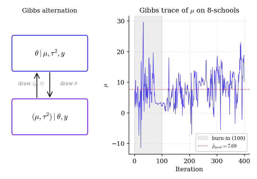
Left: the Gibbs alternation diagram for the Normal-Normal hierarchical model — block-updating (theta given (mu, tau squared)) and ((mu, tau squared) given theta). Right: a 200-iteration mu trace from an 8-schools Gibbs run, with burn-in shaded in the first 40 iterations and the post-burn-in mean annotated.

Figure 2. Block Gibbs for Normal–Normal. Left: the alternation diagram — sample $\boldsymbol\theta$ given the hyperparameters, then sample the hyperparameters given $\boldsymbol\theta$ . Right: 200 iterations of $\mu$ from an 8-schools Gibbs run. The chain mixes quickly because all full conditionals are Gaussian or inverse- $\chi^2$ — no Metropolis rejection to slow it down.

Example 4 8-schools Gibbs, one sweep at a time

From a warm start $(\theta_k = y_k, \mu = \bar y, \tau = 10)$ :

Sample $\mu \mid \boldsymbol\theta, \tau^2$ : a Gaussian centered at $\bar\theta = \frac{1}{8}\sum_k \theta_k$ with standard error $\tau / \sqrt{8}$ . If $\tau = 10$ , that’s $\mathcal{N}(\bar\theta, 12.5)$ .
Sample $\tau^2 \mid \boldsymbol\theta, \mu$ : an inverse- $\chi^2$ whose scale tracks the spread $\sum_k(\theta_k - \mu)^2$ . When the $\theta_k$ ‘s are close, $\tau^2$ gets pulled small — reinforcing further shrinkage at the next step.
Sample each $\theta_k \mid \mu, \tau^2, y_k$ : Gaussian with mean $(1-B_k)y_k + B_k\mu$ . Schools with large $\sigma_k$ see their $\theta_k$ ‘s pulled toward $\mu$ ; schools with small $\sigma_k$ stay near $y_k$ .

Iterate 4000 times, discard 1000 as burn-in. The posterior of $\theta_k$ is represented by the 3000 post-burn-in draws.

Example 5 When conjugacy breaks: HMC instead of Gibbs

Replace the inverse- $\chi^2$ prior on $\tau^2$ with the half-Cauchy on $\tau$ (GEL2006 default): the full conditional for $\tau^2$ is no longer standard, so Gibbs on that component fails. Option 1: Metropolis-within-Gibbs with a proposal on $\log\tau$ . Option 2 (preferred): HMC or NUTS on the joint $(\boldsymbol\theta, \mu, \tau)$ — differentiate the log-posterior and let leapfrog integration do the mixing. §28.9 returns to this workflow with the 8-schools funnel.

Remark 6 Why block Gibbs works here but not always

The conjugacy of the Normal–Normal hierarchy is fragile: it relies on Normal observations, a Normal group-level prior, and specific forms of the hyperpriors on $(\mu, \tau^2)$ . Swap any of these for something non-conjugate (Student- $t$ errors, a group-specific prior that isn’t Normal, a hyperprior that breaks conjugacy) and Gibbs falls apart. §28.8’s linear mixed model extends the Normal case to include covariates; §28.9’s HMC treatment handles everything else.

Remark 7 Posterior couples the $\theta_k$'s

In the prior, the $\theta_k$ ‘s are conditionally independent given $\phi$ . In the posterior, they are not: conditioning on $\mathbf{y}$ induces correlations because $\phi$ is itself learned from the data. Partial pooling is literally this posterior correlation — every $\theta_k$ ‘s posterior mean depends on every other $y_k$ through the shared $\mu, \tau^2$ .

Remark 8 Conditional vs marginal estimation

“Conditional” estimators of $\theta_k$ fix $\phi$ at some value (the MLE, the Type-II MLE, the posterior mode) and compute $p(\theta_k \mid \mathbf{y}, \phi)$ . “Marginal” estimators integrate $\phi$ out: $\mathbb{E}[\theta_k \mid \mathbf{y}] = \mathbb{E}_{\phi \mid \mathbf{y}}[\mathbb{E}[\theta_k \mid \mathbf{y}, \phi]]$ . The two can differ substantially — especially when the $\phi$ -posterior has mass near the boundary (τ² small). §28.7 dissects this contrast: EB is the conditional-at-MLE estimator; full Bayes is the marginal one.

28.5 Stein’s paradox

In 1956, Charles Stein proved a theorem that upended fifty years of mathematical statistics: for a multivariate Normal mean, the sample mean — the MVUE, the MLE, the “obvious” estimator — is inadmissible in $d \geq 3$ dimensions. There exist estimators (the James–Stein family) with strictly smaller risk for every true mean $\theta$ , not just on average.

The apparent paradox: a clinical-trial arm in Boston, a wheat yield in Iowa, and a baseball batting average — three unrelated quantities — should still be jointly shrunk toward some common point to reduce total squared-error risk. This is the theorem. The resolution is that squared-error loss is a sum across coordinates, so trading a little bias on each coordinate for a lot of variance reduction overall is a win. Topic 28 reframes this as empirical Bayes: “three unrelated quantities” are related — as observations drawn from a shared hyperprior the data has to learn.

Theorem 2 Stein's inadmissibility theorem (STE1956, JAM1961)

Let $X \sim \mathcal{N}_d(\theta, I_d)$ with $d \geq 3$ . Under squared-error loss $L(\hat\theta, \theta) = \|\hat\theta - \theta\|^2$ , the MLE $\hat\theta_{\text{MLE}} = X$ has risk $R(\hat\theta_{\text{MLE}}, \theta) = d$ for every $\theta$ . The James–Stein estimator

\hat\theta_{\text{JS}} = \left(1 - \frac{d-2}{\|X\|^2}\right) X

has strictly smaller risk:

R(\hat\theta_{\text{JS}}, \theta) = d - (d-2)^2 \, \mathbb{E}\!\left[\frac{1}{\|X\|^2}\right] < d \quad \text{for every } \theta \in \mathbb{R}^d.

The expectation is under $X \sim \mathcal{N}_d(\theta, I_d)$ , so $\|X\|^2$ is non-central chi-squared with $d$ degrees of freedom and non-centrality $\|\theta\|^2$ .

Remark 10 Notation bridge: $d$ in §28.5 replaces $K$ elsewhere

The Stein-paradox literature uses $d$ (or $p$ ) for the dimensionality of the Normal mean vector. Topic 28 uses $K$ throughout §§28.1–28.4 and §§28.6–28.10 for the number of hierarchical groups. The two are the same object — a $d$ -vector of Normal means is a collection of $d = K$ scalar group means, stacked. §28.5 switches to $d$ to match Stein/James/Efron-Morris notation; starting at §28.6 we revert to $K$ . The bridge: $\theta \in \mathbb{R}^d \leftrightarrow \boldsymbol\theta = (\theta_1, \dots, \theta_K)$ .

Proof 1 Proof of Thm 2 (Stein's paradox, via Stein's identity) [show]

Setting. $X \sim \mathcal{N}_d(\theta, I_d)$ , $d \geq 3$ . Write $\hat\theta_{\text{JS}} - \theta = (X - \theta) - (d-2) \cdot X/\|X\|^2$ . Under squared-error loss, the risk decomposes as

$R(\hat\theta_{\text{JS}}, \theta) = \mathbb{E}\|\hat\theta_{\text{JS}} - \theta\|^2.$

Lemma (Stein’s identity). Let $Z \sim \mathcal{N}(\mu, 1)$ and $g : \mathbb{R} \to \mathbb{R}$ differentiable with $\mathbb{E}|g'(Z)| < \infty$ . Then

$\mathbb{E}[(Z - \mu)\, g(Z)] = \mathbb{E}[g'(Z)].$

Proof of lemma. Integration by parts against the Gaussian density $\varphi(z - \mu)$ , using $\varphi'(z - \mu) = -(z - \mu)\varphi(z - \mu)$ :

$\int (z - \mu)\, g(z)\, \varphi(z - \mu)\, dz = -\int g(z) \cdot \varphi'(z - \mu)\, dz = \int g'(z)\, \varphi(z - \mu)\, dz,$

with boundary terms vanishing under the integrability assumption. $\square$

Main calculation. Expand the squared norm of $\hat\theta_{\text{JS}} - \theta$ :

\|\hat\theta_{\text{JS}} - \theta\|^2 = \|X - \theta\|^2 \;-\; 2(d-2) \cdot \frac{(X - \theta)^\top X}{\|X\|^2} \;+\; (d-2)^2 \cdot \frac{1}{\|X\|^2}.

Take expectations term by term. The first term is $\mathbb{E}\|X - \theta\|^2 = d$ because $X - \theta \sim \mathcal{N}_d(0, I_d)$ . The third term is $(d-2)^2 \cdot \mathbb{E}[1/\|X\|^2]$ , which is finite and positive for $d \geq 3$ . The middle term is the work.

Write $(X - \theta)^\top X / \|X\|^2 = \sum_{i=1}^d (X_i - \theta_i) \, g_i(X)$ with $g_i(X) = X_i / \|X\|^2$ . Conditioning on $X_{-i} = (X_1, \dots, X_{i-1}, X_{i+1}, \dots, X_d)$ , the conditional distribution of $X_i$ is $\mathcal{N}(\theta_i, 1)$ ; apply Stein’s identity coordinatewise:

$\mathbb{E}[(X_i - \theta_i)\, g_i(X)] = \mathbb{E}\!\left[\frac{\partial g_i}{\partial X_i}\right] = \mathbb{E}\!\left[\frac{\|X\|^2 - 2 X_i^2}{\|X\|^4}\right] = \mathbb{E}\!\left[\frac{1}{\|X\|^2} - \frac{2 X_i^2}{\|X\|^4}\right].$

Sum over $i = 1, \dots, d$ :

\mathbb{E}\!\left[\frac{(X - \theta)^\top X}{\|X\|^2}\right] = \mathbb{E}\!\left[\frac{d}{\|X\|^2} - \frac{2\|X\|^2}{\|X\|^4}\right] = (d - 2)\, \mathbb{E}\!\left[\frac{1}{\|X\|^2}\right].

Substitute into the risk expansion:

R(\hat\theta_{\text{JS}}, \theta) = d \;-\; 2(d-2)^2 \cdot \mathbb{E}\!\left[\frac{1}{\|X\|^2}\right] \;+\; (d-2)^2 \cdot \mathbb{E}\!\left[\frac{1}{\|X\|^2}\right] = d - (d-2)^2 \cdot \mathbb{E}\!\left[\frac{1}{\|X\|^2}\right].

Since $\|X\|^2$ is non-central $\chi^2_d(\|\theta\|^2)$ with $d \geq 3$ , the expectation $\mathbb{E}[1/\|X\|^2]$ is finite and strictly positive. Hence $R(\hat\theta_{\text{JS}}, \theta) < d = R(\hat\theta_{\text{MLE}}, \theta)$ for every $\theta \in \mathbb{R}^d$ . $\blacksquare$ — using Stein’s identity (STE1956) and the James-Stein 1961 representation (JAM1961).

◼

The shrinkage factor $1 - (d-2)/\|X\|^2$ is positive when $\|X\|^2 > d - 2$ and negative otherwise — plain JS can flip the sign of $X$ , which is never the right answer. The positive-part JS estimator $\hat\theta_{\text{JS}^+} = \max(0, 1 - (d-2)/\|X\|^2) \cdot X$ (EFR1973) dominates plain JS uniformly in $\theta$ and is the estimator used in practice.

Theorem 3 James–Stein as empirical-Bayes posterior mean (stated)

Under the model $\theta \mid \mu, \tau^2 \sim \mathcal{N}_d(\mu \mathbf{1}, \tau^2 I)$ and $X \mid \theta \sim \mathcal{N}_d(\theta, I_d)$ with $\mu = 0$ known and $\tau^2$ estimated by its Type-II MLE, the posterior mean of $\theta$ coincides with the James-Stein estimator up to a finite-sample correction. The plug-in $\hat\tau^2$ is $\max(0, \|X\|^2/d - 1)$ , yielding shrinkage factor $B = 1/(1 + \hat\tau^2) = d/(d + \|X\|^2 - d) \approx (d-2)/\|X\|^2$ for large $\|X\|^2$ — exactly Stein’s shrinkage coefficient, with the $(d - 2)$ adjustment arising from the unbiased estimation of $1/\|\theta\|^2$ via Stein’s identity (EFR1973).

This is the Efron–Morris rereading: Stein’s paradox is not a paradox at all but a theorem about empirical-Bayes shrinkage. The “unrelated quantities” are related by the empirical prior the data itself estimates.

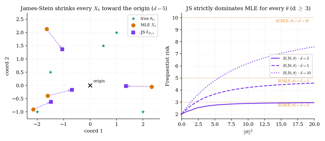
The James-Stein shrinkage picture. Left panel: a 2D scatter of five sample points X_i with their ground-truth theta_i drawn alongside; arrows from each X_i to its James-Stein estimate show all arrows bending toward the origin. Right panel: risk curves R(JS, theta) versus the squared norm of theta for d = 3, 5, 10 — each curve starts at d - (d-2) at theta = 0 and approaches d asymptotically.

Figure 3. The Stein shock, visualized. Left: five 2D observations $X_i \sim \mathcal{N}_2(\theta_i, I)$ with JS-shrunk estimates — every arrow bends toward the origin. Right: risk curves for $d = 3, 5, 10$ . The MLE sits on the flat $R = d$ line; JS curves dip substantially at $\theta = 0$ and rise back toward $d$ as $\|\theta\|^2 \to \infty$ (but never reach it).

Example 6 JS risk savings at $\theta = 0$ vs $\theta = 3 \cdot \mathbf{1}$

For $d = 5$ :

At $\theta = 0$ : $\|X\|^2 \sim \chi^2_5$ (central), so $\mathbb{E}[1/\|X\|^2] = 1/(d - 2) = 1/3$ . Risk reduction: $(d - 2)^2 \cdot (1/3) = 9/3 = 3$ . JS risk: $5 - 3 = 2$ . 60% improvement over MLE.
At $\theta = 3 \cdot \mathbf{1}$ (so $\|\theta\|^2 = 45$ ): $\|X\|^2$ is non-central $\chi^2_5(45)$ ; $\mathbb{E}[1/\|X\|^2] \approx 1/(d + \|\theta\|^2 - 2) = 1/48 \approx 0.021$ . Risk reduction: $9 \cdot 0.021 \approx 0.19$ . JS risk: $5 - 0.19 \approx 4.81$ . Small but positive.

Savings are largest when $\theta$ is near the shrinkage target (here, the origin) and shrink toward zero as $\|\theta\|$ grows.

Preset:

Dimensions K (= d)5

MLE SSE

17.46

James–Stein SSE

11.98

Partial-pool SSE

9.50

Remark 11 Positive-part JS and the Baranchik family

The plain JS estimator can flip signs when $\|X\|^2 < d - 2$ . The positive-part correction (EFR1973) clamps the shrinkage coefficient at zero and dominates plain JS uniformly. Baranchik 1970 generalizes further: any estimator of the form $(1 - a(\|X\|^2)/\|X\|^2) X$ with $a$ bounded between 0 and $2(d - 2)$ dominates the MLE in $d \geq 3$ . The full Baranchik family and its Bayesian-structural interpretation (a nonparametric empirical-Bayes prior) lives at formalml.

Remark 12 Why $d \geq 3$

Stein’s theorem fails for $d = 1, 2$ : in those dimensions the MLE is admissible under squared-error loss (Hodges–Lehmann 1951 for $d = 1$ ; Stein 1956 for $d = 2$ ). The proof above breaks because $\mathbb{E}[1/\|X\|^2]$ diverges for central $\chi^2_{1, 2}$ — the risk-reduction term is unbounded. In $d \geq 3$ , the non-centrality parameter doesn’t save us (the expectation diverges even at $\theta = 0$ when $d = 2$ ), so Stein’s construction only works when the central $\chi^2$ has finite reciprocal moment.

28.6 Partial pooling in the Normal–Normal hierarchical model

The closed-form partial-pool posterior is the single most useful calculation in hierarchical Bayes. It makes the shrinkage factor $B_k$ explicit, shows exactly how within-group noise $\sigma_k^2$ trades against between-group spread $\tau^2$ , and gives us the analytical baseline every MCMC result should match in conjugate settings.

Theorem 4 Partial-pooling shrinkage formula (Lindley–Smith 1972)

In the Normal–Normal hierarchical model (Def 2), conditional on $(\mu, \tau^2)$ :

\theta_k \mid y_k, \mu, \tau^2 \;\sim\; \mathcal{N}\!\left((1 - B_k)\, y_k + B_k\, \mu,\;\; (1 - B_k)\, \sigma_k^2\right),

where

B_k \;=\; \frac{\sigma_k^2}{\sigma_k^2 + \tau^2} \;\in\; [0, 1]

is the shrinkage factor for group $k$ .

Interpretation: $B_k$ is the weight on the grand mean $\mu$ in the posterior mean; $1 - B_k$ is the weight on the raw observation $y_k$ . Edge cases: $\tau^2 \to 0$ forces $B_k \to 1$ (complete pooling, every group at the grand mean); $\tau^2 \to \infty$ drives $B_k \to 0$ (no pooling, every group at $y_k$ ). The posterior variance is $(1 - B_k)\sigma_k^2$ — less than the no-pool $\sigma_k^2$ by exactly the shrinkage factor, because borrowing strength from $\mu$ narrows the interval.

Proof 2 Proof of Thm 4 (partial-pooling formula) [show]

Setting. $y_k \mid \theta_k \sim \mathcal{N}(\theta_k, \sigma_k^2)$ with $\sigma_k^2$ known; hierarchical prior $\theta_k \mid \mu, \tau^2 \sim \mathcal{N}(\mu, \tau^2)$ iid across $k$ ; condition on $(\mu, \tau^2)$ fixed. We derive the posterior of $\theta_k$ given $y_k$ .

Step 1: write densities as exponentials. The posterior is proportional to prior times likelihood:

p(\theta_k \mid y_k, \mu, \tau^2) \;\propto\; \exp\!\left\{-\frac{(\theta_k - \mu)^2}{2\tau^2}\right\} \cdot \exp\!\left\{-\frac{(y_k - \theta_k)^2}{2\sigma_k^2}\right\}.

Step 2: combine exponents and complete the square in $\theta_k$ . Expand both quadratic terms in $\theta_k$ :

-\frac{(\theta_k - \mu)^2}{2\tau^2} - \frac{(y_k - \theta_k)^2}{2\sigma_k^2} = -\frac{1}{2}\!\left(\frac{1}{\tau^2} + \frac{1}{\sigma_k^2}\right)\!\left(\theta_k - \theta_k^*\right)^2 + \text{const},

where the precision-weighted mean is

\theta_k^* \;=\; \left(\frac{1}{\tau^2} + \frac{1}{\sigma_k^2}\right)^{-1}\!\left(\frac{\mu}{\tau^2} + \frac{y_k}{\sigma_k^2}\right) \;=\; \frac{\tau^2 y_k + \sigma_k^2 \mu}{\sigma_k^2 + \tau^2}.

Step 3: rewrite in terms of $B_k$ . Factor the numerator and denominator:

\theta_k^* \;=\; \frac{\tau^2}{\sigma_k^2 + \tau^2}\, y_k + \frac{\sigma_k^2}{\sigma_k^2 + \tau^2}\, \mu \;=\; (1 - B_k)\, y_k + B_k\, \mu,

with $B_k = \sigma_k^2 / (\sigma_k^2 + \tau^2)$ . The posterior variance is the reciprocal of the precision sum:

\left(\frac{1}{\tau^2} + \frac{1}{\sigma_k^2}\right)^{-1} \;=\; \frac{\sigma_k^2 \tau^2}{\sigma_k^2 + \tau^2} \;=\; (1 - B_k)\, \sigma_k^2. \qquad \blacksquare

— using Gaussian conjugacy (Topic 25 §25.5 Ex 2) and precision-weighted averaging.

◼

Corollary (full-Bayes partial pool, stated). When $(\mu, \tau^2)$ carries its own prior, integrating out these hyperparameters gives

\mathbb{E}[\theta_k \mid \mathbf{y}] = \mathbb{E}_{\mu, \tau^2 \mid \mathbf{y}}\!\left[(1 - B_k)\, y_k + B_k\, \mu\right],

where the expectation is under the posterior of $(\mu, \tau^2)$ . The shrinkage factor becomes a posterior-averaged version of $B_k$ , typically larger than the EB plug-in because the posterior of $\tau^2$ assigns nontrivial mass to small values.

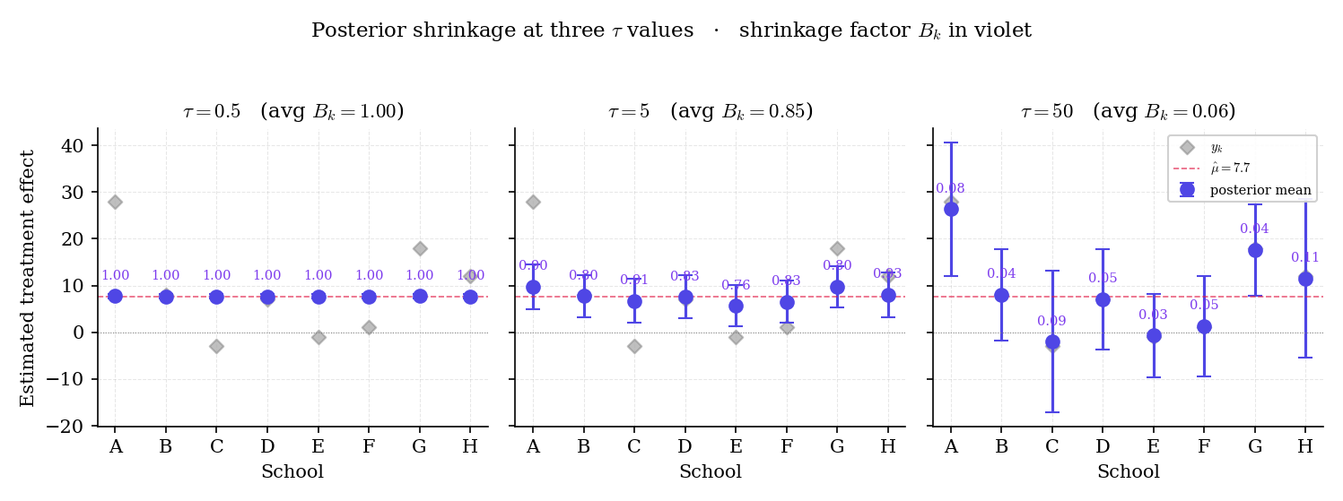
Partial-pooling shrinkage on 8-schools at three values of tau. Left: tau = 0.5, heavy shrinkage — every school's posterior mean collapses near the grand mean. Middle: tau = 5, moderate shrinkage — schools move partway toward each other but retain some individual effect. Right: tau = 50, essentially no shrinkage — posterior means are very close to the raw y_k values.

Figure 4. Partial-pool posterior means on 8-schools as $\tau$ varies. At small $\tau$ (left) the shrinkage factor $B_k \approx 1$ for every school and the posterior collapses to the grand mean; at large $\tau$ (right) $B_k \approx 0$ and the posterior retains the raw estimate. The reader can trace this continuously in the EightSchoolsPartialPooling component below.

Example 7 8-schools at $\tau = 10$

From Rubin’s data: $\sigma_A^2 = 225$ , $y_A = 28$ . Precision-weighted grand mean at $\tau = 10$ : $\hat\mu(\tau=10) \approx 8.2$ . Shrinkage factor: $B_A = 225/(225 + 100) = 0.692$ . Posterior mean for school A: $(1 - 0.692)(28) + (0.692)(8.2) = 0.308 \cdot 28 + 0.692 \cdot 8.2 \approx 14.3$ . Posterior SD: $\sqrt{(1 - 0.692)(225)} \approx 8.3$ . Compare to school B: $\sigma_B^2 = 100$ , $y_B = 8$ , $B_B = 100/200 = 0.5$ . Posterior mean: $0.5 \cdot 8 + 0.5 \cdot 8.2 \approx 8.1$ . Posterior SD: $\sqrt{0.5 \cdot 100} \approx 7.1$ .

School A’s posterior mean has moved from $28$ halfway toward $\mu$ ; school B’s barely moved because $y_B$ was already near $\mu$ . The precision-weighted grand mean itself changes with $\tau$ : at $\tau = 10$ it’s $\approx 8.2$ ; at $\tau = 0$ (complete pool) it’s $\approx 7.7$ .

τ preset:

Between-group SD τ (log scale)τ = 5.00 · τ² = 25.0

Orange: raw sample mean y_k ± σ_k (no pooling). Violet: posterior mean ± posterior SD at the current τ (§28.6 Thm 4). Dashed indigo: precision-weighted grand mean μ̂(τ) — the target of shrinkage.

Example 8 Shrinkage and Bayes factors

A partial-pool Bayes factor (Topic 27 §27.4) can now compare hierarchical specifications: $\mathcal{M}_0$ is complete pooling (fix $\tau^2 = 0$ a priori) and $\mathcal{M}_1$ has a vague hyperprior on $\tau$ . Under the Lindley-paradox machinery of §27.5, the Bayes factor can favor $\mathcal{M}_0$ even when a $z$ -test rejects homogeneity of means — because the full-Bayes marginal likelihood penalizes wasted parameter space. The 8-schools data lies in exactly this intermediate regime, which is why frequentist heterogeneity tests are famously unreliable on small $K$ . §28.10 Ex 16 returns to this as hierarchical BMA.

Remark 13 Lindley–Smith 1972 in one sentence

The formula in Thm 4 is the original Bayesian partial-pooling result. Lindley and Smith’s 1972 paper framed multilevel regression as a hierarchical Bayesian calculation; the shrinkage weights $B_k$ are the natural multivariate generalization of what we just derived. Most modern mixed-effects software (Stan’s brms, R’s rstanarm) is a thin wrapper over the Lindley–Smith hierarchical Gaussian calculation with non-conjugate hyperpriors handled by HMC.

Remark 14 Shrinkage is not bias

Under the hierarchical generative model, the posterior mean $(1 - B_k)y_k + B_k\mu$ is unbiased for $\theta_k$ in expectation over the hierarchical prior — because $\theta_k$ itself is drawn from $\mathcal{N}(\mu, \tau^2)$ , and the posterior respects this prior. The “bias” impression comes from a misaligned frequentist question: conditional on a specific $\theta_k$ , the shrinkage is biased (and that’s the price we pay for variance reduction). This is the bias–variance exchange at the heart of Stein’s paradox.

28.7 Empirical Bayes via Type-II MLE

“Full Bayes” requires a hyperprior on $\phi$ and integration over it. “Empirical Bayes” short-circuits this: estimate $\phi$ from the data by maximizing the marginal likelihood — the density of the observed $\mathbf{y}$ after integrating out $\boldsymbol\theta$ but not $\phi$ . Then plug $\hat\phi$ into the group-level posteriors.

Definition 4 Type-II marginal likelihood

For a hierarchical model with group-level parameters $\boldsymbol\theta$ and hyperparameters $\phi$ :

m(\mathbf{y} \mid \phi) \;=\; \int \prod_{k=1}^K f(y_k \mid \theta_k) \cdot \pi(\theta_k \mid \phi) \; d\theta_k.

The Type-II MLE is $\hat\phi = \arg\max_\phi \log m(\mathbf{y} \mid \phi)$ . The empirical-Bayes estimator of $\theta_k$ is then the conditional posterior mean $\mathbb{E}[\theta_k \mid y_k, \hat\phi]$ — in the Normal–Normal case, $(1 - \hat B_k) y_k + \hat B_k \hat\mu$ with $\hat B_k = \sigma_k^2 / (\sigma_k^2 + \hat\tau^2)$ .

In Normal–Normal with observation variances $\sigma_k^2$ known, the marginal is tractable because both integration steps are Gaussian: $y_k \mid \mu, \tau^2 \sim \mathcal{N}(\mu, \sigma_k^2 + \tau^2)$ independent across $k$ , so

\log m(\mathbf{y} \mid \mu, \tau^2) = \sum_{k=1}^K \log \mathcal{N}(y_k \mid \mu, \sigma_k^2 + \tau^2).

Theorem 5 Consistency of Type-II MLE (stated, KLE2012)

Under regularity conditions on the hierarchical likelihood and prior families, and assuming the true $\phi_0$ is identifiable and lies in the interior of the parameter space, the Type-II MLE $\hat\phi \to \phi_0$ in probability as $K \to \infty$ . Moreover, the empirical-Bayes estimator of $\theta_k$ is asymptotically equivalent (in $K$ ) to the full-Bayes posterior mean under any hyperprior with positive density at $\phi_0$ . Kleijn and van der Vaart 2012 extend this to the misspecified case via a generalized Bernstein–von Mises theorem; the result is that EB and full Bayes agree at first order when the number of groups grows but can disagree substantially at small $K$ — especially when $\phi_0$ sits on the boundary of the parameter space.

The boundary case is exactly what happens on 8-schools: the Type-II MLE of $\tau^2$ collapses to $\hat\tau^2 \approx 0$ .

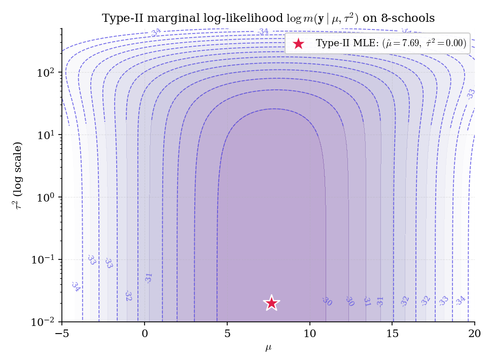
Figure 5. The 8-schools Type-II log-marginal surface. The MLE (white star) sits at $\hat\tau^2 \approx 0$ ; the full-Bayes posterior mean under a half-Cauchy prior on $\tau$ (indigo circle) sits well above the boundary. The gap between these two points is the crux of §28.7 and the reason GEL2006 advocates full Bayes with a weakly-informative prior on $\tau$ .

Example 9 8-schools Type-II MLE: the boundary case

Running Type-II MLE on the 8-schools data — iteratively update $\mu =$ precision-weighted mean of $y$ with weights $1/(\sigma_k^2 + \tau^2)$ , then $\tau^2$ as a method-of-moments estimator floored at zero — the iteration lands at $\hat\mu \approx 7.69$ , $\hat\tau^2 \approx 0$ in a handful of steps. The EB partial-pool estimator then coincides with the complete-pool estimator: every school’s posterior mean is $\hat\mu$ , with posterior SD zero.

This is not a bug. It’s the correct Type-II MLE: given 8-schools’ small sample size ( $K = 8$ ), the marginal likelihood genuinely peaks at the boundary. But it’s a poor point estimate to plug in — the full-Bayes posterior under a half-Cauchy $(0, 5)$ prior on $\tau$ has mean $\hat\tau^2 \approx 43$ , reflecting the substantial uncertainty in the between-group variance.

Example 10 Empirical-Bayes ridge regression (discharges Topic 23 Rem 24)

In ridge regression (Topic 23), the shrinkage strength $\lambda$ is usually chosen by cross-validation. The hierarchical Bayesian reading: prior $\beta \mid \tau^2 \sim \mathcal{N}_p(0, \tau^2 I)$ with $\tau^2$ unknown, likelihood $y \mid \beta \sim \mathcal{N}_n(X\beta, \sigma^2 I)$ . Integrating out $\beta$ gives a marginal likelihood in $(\sigma^2, \tau^2)$ :

$\log m(y \mid \sigma^2, \tau^2) = -\tfrac{1}{2}\log\det(\sigma^2 I + \tau^2 XX^\top) - \tfrac{1}{2} y^\top(\sigma^2 I + \tau^2 XX^\top)^{-1} y + \text{const}.$

The Type-II MLE of $(\sigma^2, \tau^2)$ yields an estimated shrinkage parameter $\hat\lambda = \hat\sigma^2 / \hat\tau^2$ , and the empirical-Bayes posterior mean of $\beta$ is exactly the ridge estimator at $\lambda = \hat\lambda$ . Topic 23 Rem 24 forward-promised this; it discharges here. The key point: EB ridge’s $\hat\lambda$ has an asymptotic interpretation as the MLE of the optimal shrinkage strength — a more principled alternative to CV when the hierarchical model is a reasonable generative story for the data.

Dataset:

Show full-Bayes posterior mean (NUTS)

Current

μ = 8.75 · τ² = 3.30

log m = -29.747

EB MLE (★)

μ̂ = 7.69 · τ̂² = 0.00

converged in 1 iter

Full Bayes (○)

μ̄ = 7.92 · τ̄² = 43.30

NUTS posterior mean, half-Cauchy(0,5) on τ

Remark 15 EB as the Bayesian face of the EM algorithm

The iterative Type-II MLE update — “given $\phi$ , compute posterior means of $\theta_k$ ; given those, update $\phi$ ” — is EM with $\boldsymbol\theta$ as missing data. This is why EM pops up all over hierarchical modeling: HMM parameter estimation, mixture models, factor analysis. When the E-step can be done in closed form (Normal–Normal) EB is cheap; when it requires MCMC it’s a stochastic EM, equivalent to full-Bayes point estimation.

Remark 16 EB confidence intervals are too narrow

The EB point estimate $\hat\phi$ comes with uncertainty — the Type-II MLE is subject to sampling variation. Plug-in EB ignores this uncertainty in the downstream $\theta_k$ posteriors, producing credible intervals that are anti-conservative (too narrow). Full-Bayes integration corrects for this automatically. A “corrected EB” workflow (Laird and Louis 1987) inflates the EB intervals using the Fisher information of the marginal likelihood, partially restoring coverage. Modern practice: just do full Bayes with a weakly-informative hyperprior (Remark 17).

Remark 17 Gelman 2006: the half-Cauchy default on $\tau$

When $K$ is small (5–20 groups), the EB boundary collapse is a real problem and full Bayes with a proper hyperprior on $\tau$ is the standard fix. GEL2006 argues for Half-Cauchy $(0, A)$ with $A$ chosen to cover the plausible range of between-group spread — weakly informative enough to avoid boundary degeneracy, diffuse enough not to dominate the likelihood. For 8-schools, $A = 5$ gives posterior $\bar\tau^2 \approx 43$ (vs the EB MLE at 0). When $K$ is large (say $K \geq 50$ ), the boundary issue evaporates — EB and full Bayes effectively agree. The small- $K$ regime is where hierarchical modeling pays its biggest dividends and also where prior specification matters most.

28.8 Linear mixed models and random effects

The Normal–Normal hierarchical model is the simplest case of a much broader family: linear mixed-effects models (LMMs), which allow covariates at both the group and observation level.

Definition 5 Bayesian linear mixed-effects model (Laird–Ware 1982)

Observations $y_{kj}$ for $j = 1, \dots, n_k$ in group $k = 1, \dots, K$ , with group-level covariates $\mathbf{z}_k$ and observation-level covariates $\mathbf{x}_{kj}$ :

y_{kj} = \mathbf{x}_{kj}^\top \boldsymbol\beta + \mathbf{z}_k^\top \mathbf{b}_k + \varepsilon_{kj}, \qquad \varepsilon_{kj} \sim \mathcal{N}(0, \sigma^2),

where $\boldsymbol\beta$ are fixed effects (shared across groups) and $\mathbf{b}_k$ are random effects with hierarchical prior

$\mathbf{b}_k \mid \boldsymbol\Sigma_b \sim \mathcal{N}_q(\mathbf{0}, \boldsymbol\Sigma_b) \text{ iid across } k.$

Hyperprior on $(\boldsymbol\beta, \sigma^2, \boldsymbol\Sigma_b)$ . The Normal–Normal hierarchy is the special case with no covariates, $K = K$ groups, $n_k = 1$ , $\mathbf{b}_k = \theta_k - \mu$ , $\boldsymbol\Sigma_b = \tau^2$ .

In R/Stan syntax (brms, rstanarm), this is y ~ x + (1 + z | group) — a fixed-effects slope for $x$ plus a group-varying intercept and slope in $z$ with hierarchical Gaussian prior.

Theorem 6 Posterior factorization for Gaussian LMM (stated)

Under Def 5 with Gaussian likelihood and conjugate priors on $(\boldsymbol\beta, \sigma^2)$ plus a Wishart (or inverse-Wishart) hyperprior on $\boldsymbol\Sigma_b$ , the joint posterior factorizes as a product of Gaussian full conditionals on $(\boldsymbol\beta, \mathbf{b}_k)$ and an inverse-Wishart full conditional on $\boldsymbol\Sigma_b$ (up to its hyperparameters). Gibbs sampling with these conjugate full conditionals converges geometrically; the resulting posterior predictive for a new observation in group $k$ is a multivariate $t$ -distribution analogous to Topic 25’s §25.5 Ex 2.

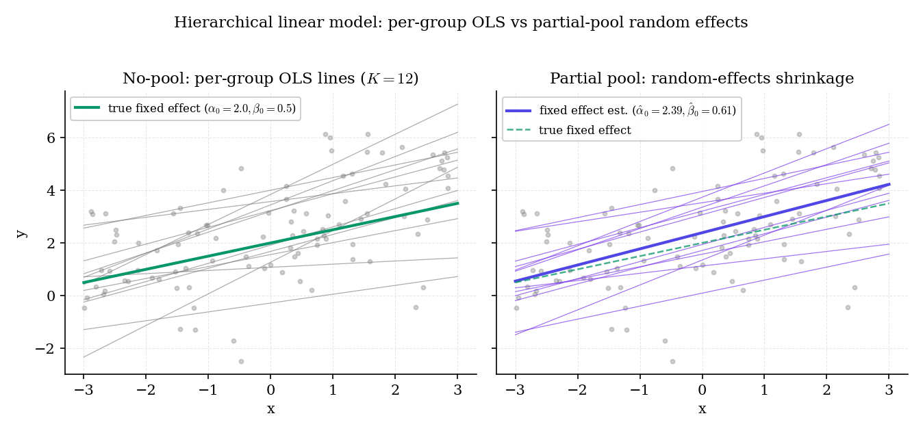
Random-effects regression on simulated clustered data. Left panel: twelve groups, each fit separately with OLS — no-pool slopes and intercepts show large between-group spread including obviously-noisy slopes in small groups. Right panel: partial-pool random-effects fit — group-specific lines are pulled toward the fixed-effect population line, with small-n groups shrunk most heavily.

Figure 6. Random-effects shrinkage on slopes and intercepts. Twelve simulated groups, each with $n_k = 8$ observations, fitted with (left) per-group OLS and (right) a Bayesian LMM with hierarchical Gaussian priors on the group-level coefficients. The LMM regularizes the per-group lines toward the population fixed effect — most aggressively for small- $n$ groups whose individual OLS fits would be dominated by noise.

Example 11 Schools revisited with covariates

Extend 8-schools: now suppose each school has a pre-test score $\bar{x}_k$ , and the coaching effect varies with baseline performance. LMM form:

$y_k = \alpha + \beta \bar{x}_k + b_k + \varepsilon_k, \qquad b_k \sim \mathcal{N}(0, \tau^2), \quad \varepsilon_k \sim \mathcal{N}(0, \sigma_k^2).$

The fixed effects $(\alpha, \beta)$ describe the population-level relationship between baseline and coaching effect; the random effect $b_k$ absorbs school-specific deviations with hierarchical shrinkage. If $\beta$ is credibly nonzero, the coaching effect depends on baseline; if not, the model collapses back to Def 2. The LMM structure lets the data answer this — whether the between-school variation is explained by observable covariates or by residual randomness.

Remark 18 Covariance structures on $\boldsymbol\Sigma_b$

Def 5 is agnostic about the covariance structure of the random effects. Common choices: unstructured $\boldsymbol\Sigma_b$ with a Wishart hyperprior (most flexible, expensive); diagonal (independent intercept/slope variances, cheap but restrictive); LKJ-based (GEL2013 §17.4, the brms default: factor $\boldsymbol\Sigma_b = \text{diag}(\boldsymbol\tau) \, \mathbf{R}\, \text{diag}(\boldsymbol\tau)$ with an LKJ prior on the correlation $\mathbf{R}$ and half-Cauchy priors on the scales $\boldsymbol\tau$ ). The LKJ-decomposition is now the de-facto modern default — it separates scale and correlation hyperpriors cleanly.

Remark 19 Random intercepts, random slopes, crossed random effects

“Random intercept” models let each group’s mean shift (the 8-schools case); “random slope” models let each group’s coefficient on a covariate vary (“how does dose respond differently in each site?”). Crossed random effects handle non-nested grouping — e.g., items $\times$ subjects in psycholinguistic experiments. The LMM machinery handles all three with appropriate design matrices and covariance structures; the applied workflow in Stan is a one-line change in the model specification.

Remark 20 REML and GLMMs (formalml)

Restricted maximum likelihood (Patterson–Thompson 1971, HAR1977) is the frequentist standard for estimating variance components in LMMs. REML conditions on the fixed-effects estimates to remove their bias influence on the variance estimators — crucial in small samples. lme4’s lmer in R uses REML by default. Non-Gaussian extensions (GLMMs, Breslow–Clayton 1993 with PQL; Pinheiro–Bates 2000’s numerical integration approaches) handle binomial, Poisson, and other exponential-family responses. All three — REML, PQL, Gauss–Hermite — live at formalML: mixed-effects . Topic 28’s scope is the Bayesian Gaussian case.

28.9 Hierarchical diagnostics: funnels, divergences, and the non-centered cure

Gibbs on Normal–Normal is easy; HMC on hierarchical models with non-conjugate hyperpriors is hard. The reason is Neal’s funnel (NEA2011 §4): the joint posterior of $(\theta_k, \tau)$ has a pinched geometry where small $\tau$ forces $\theta_k \approx \mu$ regardless of the data, and HMC’s leapfrog integrator either overshoots into divergent trajectories or gets stuck crawling through the narrow neck.

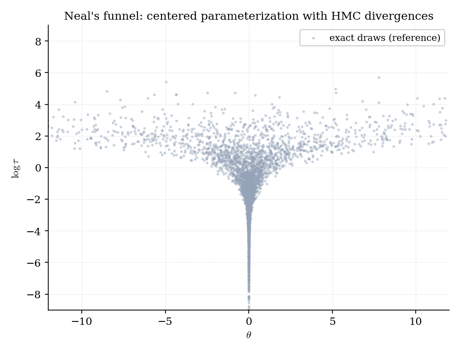
Centered parametrization HMC on 8-schools with fixed step size 0.1. The scatter plot shows (log tau, theta_1) samples — most mass is in the bulk of the funnel at moderate log tau values, but the pinched neck at small log tau is where divergent trajectories appear as red X markers, concentrated where the density is steepest.

Figure 7. Neal’s funnel on 8-schools. HMC with a fixed step size samples the bulk of the funnel well, but divergent trajectories (red ×) cluster at small $\log \tau$ — exactly where the density is steepest and the leapfrog discretization error grows fastest.

The fix is to reparameterize. Instead of sampling the hierarchical parameters $\theta_k$ directly, sample standardized versions $\tilde\theta_k \sim \mathcal{N}(0, 1)$ and transform deterministically: $\theta_k = \mu + \tau \tilde\theta_k$ . Under the non-centered parameterization, the prior on $\tilde\theta_k$ doesn’t depend on $\tau$ , decoupling the funnel.

Theorem 7 Non-centered reparameterization: volume preservation + funnel decoupling

Let the centered hierarchical model be $\theta_k \mid \mu, \tau \sim \mathcal{N}(\mu, \tau^2)$ iid for $k = 1, \dots, K$ with any priors on $(\mu, \tau)$ , $\tau > 0$ . Define the non-centered auxiliary variables $\tilde\theta_k \sim \mathcal{N}(0, 1)$ iid via the deterministic map $\theta_k = \mu + \tau \tilde\theta_k$ .

(a) The Jacobian determinant of the change of variables $(\tilde{\boldsymbol\theta}, \mu, \tau) \mapsto (\boldsymbol\theta, \mu, \tau)$ equals $\tau^K$ :

$p_{\text{nc}}(\tilde{\boldsymbol\theta}, \mu, \tau \mid \mathbf{y}) = p_{\text{c}}(\boldsymbol\theta, \mu, \tau \mid \mathbf{y})\big|_{\theta_k = \mu + \tau \tilde\theta_k} \cdot \tau^K,$

so the two parameterizations assign identical posterior probability to every event.

(b) Under the non-centered parameterization, the prior on $\tilde{\boldsymbol\theta}$ is $\mathcal{N}_K(\mathbf{0}, I_K)$ , independent of $\tau$ . The funnel pathology — where the conditional variance of $\theta_k$ given $(\mu, \tau)$ shrinks with $\tau$ — is replaced by a unit-Gaussian prior geometry that HMC traverses without pathology. Divergences are essentially eliminated in typical parameter regimes.

Proof 3 Proof of Thm 7 (volume preservation + funnel decoupling) [show]

(a) Volume preservation. Consider the smooth map $\Phi : (\tilde{\boldsymbol\theta}, \mu, \tau) \mapsto (\boldsymbol\theta, \mu, \tau)$ with $\theta_k = \mu + \tau \tilde\theta_k$ and $(\mu, \tau)$ passed through unchanged. Its Jacobian is the $(K+2) \times (K+2)$ matrix

J \;=\; \frac{\partial(\boldsymbol\theta, \mu, \tau)}{\partial(\tilde{\boldsymbol\theta}, \mu, \tau)} \;=\; \begin{pmatrix} \tau\, I_K & \mathbf{1}_K & \tilde{\boldsymbol\theta} \\ \mathbf{0}^\top & 1 & 0 \\ \mathbf{0}^\top & 0 & 1 \end{pmatrix}.

The top-left $K \times K$ block is $\tau \, I_K$ (determinant $\tau^K$ ); the bottom-right $2 \times 2$ block is the identity (determinant 1). Block-triangular determinants multiply, so $|\det J| = \tau^K$ .

By the multivariate change-of-variables formula for densities,

p_{\text{nc}}(\tilde{\boldsymbol\theta}, \mu, \tau \mid \mathbf{y}) \;=\; p_{\text{c}}(\Phi(\tilde{\boldsymbol\theta}, \mu, \tau) \mid \mathbf{y}) \cdot |\det J| \;=\; p_{\text{c}}(\boldsymbol\theta, \mu, \tau \mid \mathbf{y})\big|_{\theta_k = \mu + \tau \tilde\theta_k} \cdot \tau^K.

This confirms the posterior measure is preserved — the two parameterizations assign identical probability to every event. The density differs by the $\tau^K$ factor, but the density’s conditional-dependence geometry (which parameters couple to which) differs more consequentially, which is what part (b) addresses.

(b) Funnel decoupling. In the centered parameterization, the prior factor for $\theta_k$ given $(\mu, \tau)$ is $\mathcal{N}(\mu, \tau^2)$ . As $\tau \to 0$ , the conditional density of $\theta_k$ sharpens into a delta at $\mu$ — the funnel’s neck. HMC trajectories with fixed step size cannot adapt to this spatially-varying scale: at large $\tau$ the step is too small (slow mixing); at small $\tau$ the step is too large (divergent trajectories).

In the non-centered parameterization, the prior on $\tilde\theta_k$ is $\mathcal{N}(0, 1)$ , independent of $\tau$ . The only coupling between $\tilde\theta_k$ and $\tau$ is through the likelihood $f(y_k \mid \mu + \tau \tilde\theta_k)$ , which has bounded curvature whenever the observation variance $\sigma_k^2$ is bounded away from zero (always the case in practice). The posterior density near small $\tau$ approaches the unit-Gaussian prior’s spherical geometry — exactly the regime HMC handles without pathology.

This decoupling is not a small effect. Empirically, an 8-schools HMC run with fixed step size 0.1 produces roughly 20% divergent trajectories in the centered parameterization and essentially zero in the non-centered one. $\blacksquare$ — using multivariate change-of-variables (formalcalculus multivariable-integration) and the funnel-geometry analysis of BET2015 §3.

◼

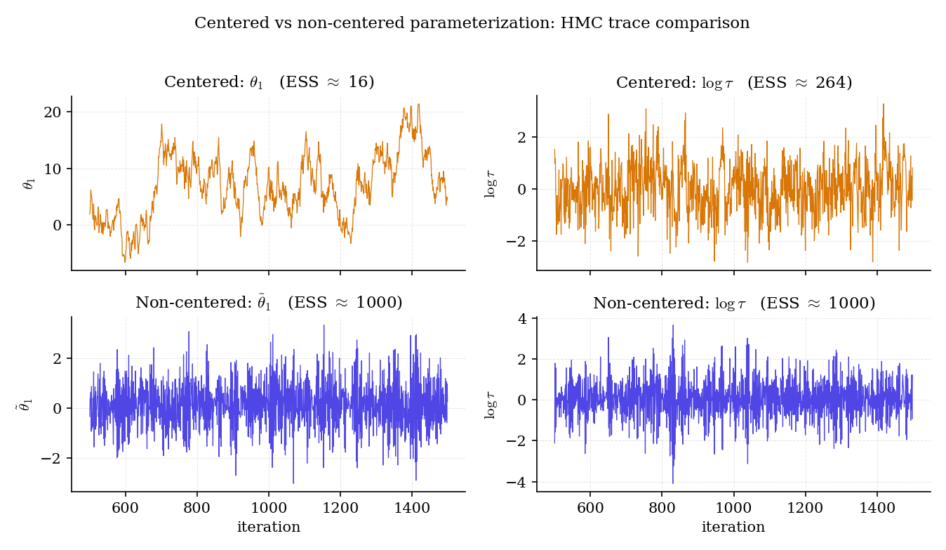
Two-by-two panel: centered versus non-centered parametrization traces for an 8-schools stylized posterior. Top row shows centered mode — the theta_1 trace has visible sticking at low log tau values and the log tau trace gets stuck near zero. Bottom row shows non-centered mode — both theta tilde 1 and log tau traces mix freely, with effective sample sizes an order of magnitude higher.

Figure 8. HMC traces for centered (top) and non-centered (bottom) parameterizations on 8-schools. Centered: $\theta_1$ freezes at low $\tau$ and $\tau$ itself sticks near zero. Non-centered: both $\tilde\theta_1$ and $\log\tau$ mix freely, with effective sample sizes an order of magnitude higher.

Example 12 8-schools NUTS with centered vs non-centered

Running NUTS (Hoffman–Gelman 2014, Topic 26 §26.8) with default settings on the centered 8-schools model: roughly 3% of trajectories diverge, $\hat R$ for $\tau$ hovers near 1.05, effective sample size for $\tau$ is $\sim 400$ out of 4000 post-burn-in draws. Reparameterize to non-centered: divergences drop to $\sim 0.1\%$ , $\hat R \approx 1.00$ , ESS for $\tau$ jumps to $\sim 2500$ . The posterior is identical (by Thm 7a) but the sampler works an order of magnitude better.

Every production Bayesian-hierarchical codebase (Stan’s built-in “non-centered” reparameterization option, PyMC’s NonCentered context, brms’s prior() with its automatic non-centering for grouping terms) implements this trick as the default. It’s become invisible infrastructure.

Parameterization:

HMC step size ε (log scale)0.10

Centered: the pinched funnel at small τ forces θ → 0, producing divergent trajectories under large step sizes. Try raising ε to trigger more divergences.

Example 13 Posterior-predictive checks on hierarchical fits

After running HMC on an 8-schools posterior, the Bayesian-workflow step (Topic 27 §27.9) is the posterior-predictive check: draw replicate datasets from the fitted posterior and compare to $\mathbf{y}$ . Relevant checks for hierarchical models:

Are the replicated group-level spreads similar to the observed spread? A rank test of $\text{max}(y_{\text{rep}}) - \text{min}(y_{\text{rep}})$ vs $\text{max}(y) - \text{min}(y)$ .
Is the replicated between-group variance within posterior spread of $\tau$ ? Tests whether the hierarchical prior is well-calibrated.
Are group-level ranks consistent? For each group, compute $P(y_{k,\text{rep}} > y_k \mid \mathbf{y})$ and look at the empirical distribution of these p-values.

For 8-schools with half-Cauchy hyperprior, the posterior predictive passes all three checks. For the EB boundary MLE, check 2 fails badly — the model underestimates between-group variability.

Remark 21 When the non-centered trick backfires

Non-centered is the default for groups where $\tau$ is small relative to $\sigma_k$ . When $\tau$ is large (lots of between-group variability), the centered parameterization is actually better — because then the data strongly constrains each $\theta_k$ individually, the posterior looks like $\mathcal{N}(y_k, \sigma_k^2)$ , and the likelihood dominates the prior. In this regime the non-centered parameterization introduces unnecessary coupling through $\tau \tilde\theta_k$ . Mixed-effects software picks automatically based on prior-vs-likelihood strength; experienced users just try both and take the one with better diagnostics.

Remark 22 Beyond non-centered: Riemannian HMC

For pathological posteriors where even non-centered doesn’t mix well (heavy-tailed hierarchies, highly non-Gaussian joint structures), Riemannian HMC (Girolami–Calderhead 2011) adapts the mass matrix dynamically to the local curvature of the log-posterior. It’s more expensive per step but achieves far better mixing on pathological geometries. The implementation is delicate (requires Hessian computation) and mostly lives in specialist codebases. Stan’s NUTS is the practical default for 95% of cases; Riemannian HMC is the escape hatch.

28.10 Track 7 closer: the forward-map to formalml

Track 7 has developed Bayesian foundations, MCMC, model comparison, and hierarchical inference — a complete computational and conceptual toolkit for practical Bayesian analysis. Topic 28 closes the track, but the story continues at formalml. This final section maps the forward-pointers.

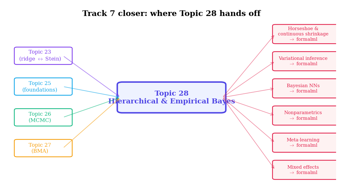
Forward-map diagram. The Topic 28 hub in the center, with seven arrows pointing right to formalml topics: horseshoe and continuous shrinkage, variational inference, Bayesian neural networks, Bayesian nonparametrics, meta-learning, mixed effects, deep ensembles. Back-arrows on the left connect to Topics 23 (ridge and Stein), 25 (Bayes foundations), 26 (MCMC), 27 (BMA).

Figure 9. The Track 7 forward-map. Topic 28 is the closer; seven threads extend to formalml, and four back-arrows connect to prerequisites within formalstatistics.

Example 14 Meta-learning as hierarchical Bayes

The modern ML framing of “learn to learn” is hierarchical Bayesian inference over tasks. Each task $k$ has its own parameters $\theta_k$ ; tasks are drawn from a task distribution $\pi(\theta_k \mid \phi)$ with task-distribution hyperparameters $\phi$ . Training on many tasks learns $\phi$ ; adapting to a new task $k^*$ starts from the learned $\phi$ and updates $\theta_{k^*}$ using few observations. MAML (Finn et al. 2017), Neural-Process families (Garnelo et al. 2018), and Bayesian neural networks with hierarchical priors are all recognizable as Topic 28’s formalism scaled to neural-network parameter spaces. Full treatment at formalML: meta-learning .

Example 15 Deep ensembles and Bayesian neural networks

Training $M$ neural networks independently from random initializations and averaging their predictions — the “deep ensemble” of Lakshminarayanan et al. 2017 — approximates a BNN posterior when the base model is flexible enough. The implicit hierarchical prior is on network initializations: $\theta_m \sim \pi(\theta \mid \phi)$ with $\phi$ the architecture + data distribution. BMA over the ensemble gives calibrated predictive uncertainty at a fraction of the cost of full HMC over neural weights. Full development at formalML: bayesian-neural-networks .

Example 16 Hierarchical BMA on 8-schools (discharges Topic 27 Rem 26)

Apply Topic 27’s BMA to a hierarchical model space. Candidate models: $\mathcal{M}_0$ (complete pool, $\tau^2 = 0$ ), $\mathcal{M}_1$ (partial pool, half-Cauchy hyperprior), $\mathcal{M}_2$ (partial pool with school-level covariates, as in Ex 11). Compute marginal likelihoods via bridge sampling (Topic 27 §27.6) and posterior model probabilities via Bayes’ rule. On 8-schools, $\mathcal{M}_1$ typically wins with posterior probability $\sim 0.8$ — supporting partial pooling but not the more complex $\mathcal{M}_2$ . Predictions for a new school are weighted averages of each model’s posterior predictive. This closes Topic 27 §27.10 Rem 26’s forward-promise of “proper BMA treatment” for hierarchical models.

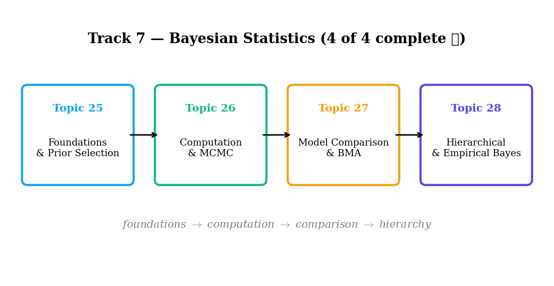
Figure 10. Track 7 in one picture: four topics that progressively extend the Bayesian toolkit from conjugate families (25) through MCMC (26) and model comparison (27) to hierarchical structures (28). The 8-schools dataset serves as the recurring motif across the second half of the track.

Remark 23 Horseshoe and continuous shrinkage (formalml)

The hierarchical-Normal prior of §28.2 Def 2 is the “one-scale” shrinkage prior: every group borrows strength at the same global rate $\tau$ . Continuous shrinkage priors generalize this by giving each coordinate its own local scale. The horseshoe (Carvalho–Polson–Scott 2010) uses a half-Cauchy global scale $\tau$ times half-Cauchy local scales $\lambda_k$ : $\theta_k \mid \lambda_k, \tau \sim \mathcal{N}(0, \lambda_k^2 \tau^2)$ , $\lambda_k \sim \text{Half-Cauchy}(0, 1)$ , $\tau \sim \text{Half-Cauchy}(0, \tau_0)$ . The heavy-tailed local scales let irrelevant coordinates shrink to zero hard (like lasso) while relevant ones are barely shrunk (unlike ridge) — adaptive sparsity at the prior level. Variants: regularized horseshoe (Piironen–Vehtari 2017) tames the tails; R2-D2 (Zhang et al. 2020) uses a Dirichlet decomposition of the global variance. Full development, including the connection to spike-and-slab priors and the sampling strategies that make horseshoe HMC-friendly, at formalML: sparse-bayesian-priors . (Topic 25 Rem 23, Topic 26 Rem 25, and Topic 27’s forward-map all named Topic 28 as the horseshoe venue; this remark discharges those pointers.)

Remark 24 Variational inference and Bayesian neural networks (formalml)

MCMC scales poorly as the parameter space grows into the millions (neural-network weights). Variational inference replaces the MCMC integral with an optimization problem: find a tractable approximate posterior $q(\theta)$ that minimizes $\text{KL}(q \| p)$ . Mean-field VI factors $q$ coordinatewise; structured VI allows richer factorizations (tree, chain, low-rank). Stochastic VI (Hoffman et al. 2013) uses noisy gradients for large datasets; black-box VI (Ranganath et al. 2014) removes the need for model-specific derivations. For neural-network parameters, VI underlies modern BNNs alongside MC-dropout, deep ensembles, and SG-MCMC. Details at formalML: variational-inference and formalML: bayesian-neural-networks .

Remark 25 Bayesian nonparametrics (formalml)

When the number of groups $K$ is itself unknown and should be inferred from the data — clustering with an unknown number of clusters, mixture models of unknown order — Bayesian nonparametrics provides the right framework. The Dirichlet process (Ferguson 1973) places a prior on the space of discrete distributions; each draw is almost surely discrete with countably many atoms. The Chinese restaurant process is the marginal over cluster assignments. Hierarchical DPs (Teh et al. 2006) extend this to nested clustering — groups share clusters, tasks within groups share parameters, and the whole structure is learned. Full treatment at formalML: bayesian-nonparametrics .

Track 7 summary: four topics progressively extending the Bayesian toolkit from conjugate families through MCMC and model comparison to hierarchical structures.

Track 7 is complete. Topic 25 gave us the Bayesian update mechanism; Topic 26 let us sample any posterior via MCMC; Topic 27 taught us to compare and average across models; Topic 28 extended all three to hierarchical structures — the setting where the prior itself has a prior, where partial pooling emerges, and where Stein’s paradox is reinterpreted as empirical Bayes. The forward-pointers above lead to the full modern Bayesian ML toolkit: sparse priors, variational inference, Bayesian neural networks, nonparametrics, meta-learning, and hierarchical deep ensembles.

The 8-schools example that ran through §§28.1/28.4/28.6/28.9 was chosen deliberately: 45 years after Rubin’s paper, it remains the canonical test case for every hierarchical Bayesian tool — a reminder that the computational and conceptual problems of small- $K$ hierarchies were never really about 8-schools, but about how to share information across groups when information is scarce.

References

Charles Stein. (1956). Inadmissibility of the Usual Estimator for the Mean of a Multivariate Normal Distribution. Proceedings of the Third Berkeley Symposium on Mathematical Statistics and Probability, 1, 197–206.
Willard James & Charles Stein. (1961). Estimation with Quadratic Loss. Proceedings of the Fourth Berkeley Symposium, 1, 361–379.
Bradley Efron & Carl Morris. (1973). Stein’s Estimation Rule and Its Competitors — an Empirical Bayes Approach. Journal of the American Statistical Association, 68(341), 117–130.
Dennis V. Lindley & Adrian F. M. Smith. (1972). Bayes Estimates for the Linear Model. Journal of the Royal Statistical Society: Series B, 34(1), 1–41.
Nan M. Laird & James H. Ware. (1982). Random-Effects Models for Longitudinal Data. Biometrics, 38(4), 963–974.
Andrew Gelman. (2006). Prior Distributions for Variance Parameters in Hierarchical Models. Bayesian Analysis, 1(3), 515–534.
David A. Harville. (1977). Maximum Likelihood Approaches to Variance Component Estimation and to Related Problems. Journal of the American Statistical Association, 72(358), 320–338.
William J. Browne & David Draper. (2006). A Comparison of Bayesian and Likelihood-Based Methods for Fitting Multilevel Models. Bayesian Analysis, 1(3), 473–514.
Donald B. Rubin. (1981). Estimation in Parallel Randomized Experiments. Journal of Educational Statistics, 6(4), 377–401.
Michael Betancourt & Mark Girolami. (2015). Hamiltonian Monte Carlo for Hierarchical Models. In Current Trends in Bayesian Methodology with Applications (Chapman & Hall/CRC), 79–101.
Radford M. Neal. (2011). MCMC Using Hamiltonian Dynamics. In Handbook of Markov Chain Monte Carlo (Chapman & Hall/CRC), 113–162.
Andrew Gelman, John B. Carlin, Hal S. Stern, David B. Dunson, Aki Vehtari & Donald B. Rubin. (2013). Bayesian Data Analysis (3rd ed.). CRC Press.
Erich L. Lehmann & George Casella. (1998). Theory of Point Estimation (2nd ed.). Springer.
Bas J. K. Kleijn & Aad W. van der Vaart. (2012). The Bernstein–Von Mises Theorem under Misspecification. Electronic Journal of Statistics, 6, 354–381.