Hidden Markov Models
Foundations of state-space inference. A finite Markov chain we never see drives every observation we do; one conditional-independence structure turns three exponential-time problems — likelihood, decoding, and learning — into linear-time passes over a trellis. Ten full proofs, featuring forward–backward smoothing; Viterbi decoding, Baum–Welch as EM with its ascent property proved, and the Kalman filter as the linear-Gaussian case. Market regimes and the dishonest casino as spine examples; speech, sequence labeling, and particle filters as the ML payoff. Track 9 opens here.
34.1 Motivation: regimes we cannot see
Look at a year or two of daily returns for almost any asset and the same pattern shows up: long, quiet stretches, then sudden bursts where every day moves a lot, then quiet again. A histogram of the returns throws that pattern away. It shows one distribution with fatter tails than a Normal, and it can’t tell us that the big moves cluster. The time order is the information. The question an ML system actually faces is a sequential one: given everything observed so far, which regime are we in today, and how sure are we?
The model this topic builds says there’s a hidden state, the market’s regime, that evolves on its own, and each day’s return is drawn from a distribution that depends only on the regime that day. We never observe the regime. We observe only its consequences. That is a hidden Markov model (HMM), and the same structure describes a speaker moving through phonemes, a genome moving between coding and non-coding stretches, a user moving between browsing and buying, or a server moving between healthy and degraded.
Take two regimes, calm and turbulent. On a calm day the return (in percent) is drawn from , a Normal distribution with mean 0.05 and standard deviation 0.7; on a turbulent day from . A calm day is followed by another calm day with probability 0.98, and a turbulent day by another turbulent day with probability 0.95. Simulating days:
- The series is turbulent on a fraction 0.362 of days. The long-run value is (Example 3 derives it), but the regimes are so persistent that 1,000 days contain only 37 switches, and the sample fraction wanders.
- The returns have sample excess kurtosis 2.77: fat tails, from a mixture of two thin-tailed Normals.
- The lag-1 autocorrelation of the returns is −0.018, essentially zero. The lag-1 autocorrelation of the squared returns is 0.206.
That last pair is the fingerprint. Returns look unpredictable, and their magnitudes are strongly predictable. Example 5 derives this in closed form.
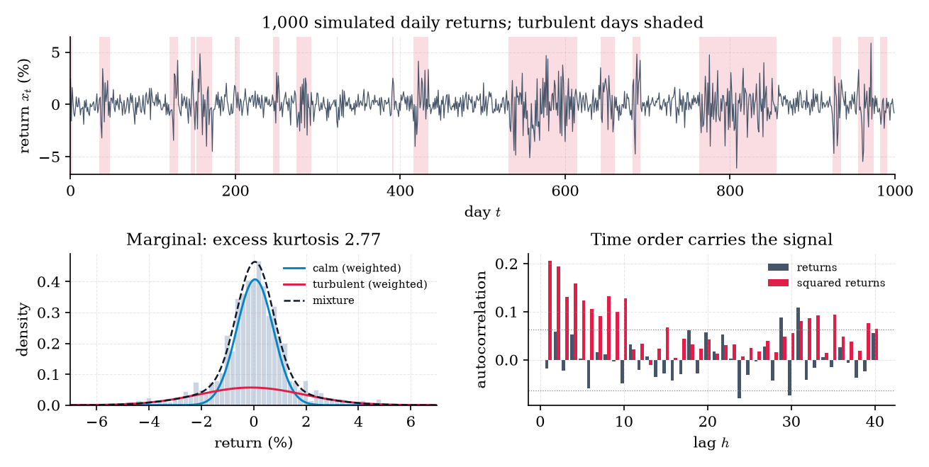
Figure 1. Two hidden regimes produce one fat-tailed histogram. The time order is the evidence: squared returns are autocorrelated even though returns are not.
A casino rolls one of two dice: a fair die and a loaded die that shows a six with probability 0.5 and each other face with probability 0.1. Between rolls it switches from the fair die to the loaded one with probability 0.05, and back with probability 0.10. We see only the 300 rolls. Which stretches were rolled with the loaded die?
We return to this example throughout §34.4–§34.6. Its emissions are dice, so every posterior probability in it has a concrete reading: “how likely is it that this roll came from the loaded die?”
We write for the hidden state at time and for the observation, with lowercase for an observed value. This matches the EM appendix of Topic 14, where was the latent label and the data. formalML’s sequential Monte Carlo page writes for the hidden state and for the observation; when crossing between the sites, swap the letters. We write for a block of consecutive observations.
Every use of an HMM reduces to one of three computations:
- Evaluate: compute the likelihood of an observed sequence (§34.4).
- Decode: recover the hidden states, either one time at a time (§34.5) or as a single best path (§34.6).
- Learn: estimate the parameters from data (§34.7).
Each has a brute-force solution that costs operations, exponential in the sequence length. The point of this topic is that the HMM’s structure brings each one down to . The picture to hold on to is the trellis: a grid with one node per (state, time) pair and edges between consecutive columns. Every algorithm here is one dynamic-programming sweep across that grid, and the only thing that changes between them is whether we sum over incoming edges or maximize over them.
34.2 Finite Markov chains
The hidden part of an HMM is a Markov chain, so we start there, but only with what HMMs need. Topic 26 developed Markov chains on general state spaces as the engine of MCMC (§26.2, §26.7); here the state space is finite and everything becomes a matrix.
A sequence taking values in is a (time-homogeneous) Markov chain if the next state depends on the past only through the present:
The transition matrix has nonnegative entries and rows that sum to 1 (it is row-stochastic): row is the distribution of the next state given the current state . The initial distribution is the row vector with . This is Topic 26’s transition kernel (§26.2 Def 1) on a finite state space.
The first fact is that multi-step behavior is matrix multiplication.
For a finite Markov chain with transition matrix and initial distribution :
(i) for all ;
(ii) , that is, ;
(iii) the marginal law of is the row vector .
Proof 1 Proof of Thm 1 (Chapman–Kolmogorov) [show]
(i) By induction on . For it is Definition 1. Suppose it holds for . Condition on with the law of total probability (Topic 2):
By the Markov property the first factor is , and by the induction hypothesis the second is . So the sum is .
(ii) is associativity of matrix multiplication, and (i) gives it a probabilistic reading: to go from to in steps, the chain passes through some state at step .
(iii) By total probability over and (i) with :
— using the law of total probability and the Markov property (Definition 1).
The second fact is that a well-behaved chain forgets where it started.
A distribution on is stationary for if : starting the chain from , every has law . Geometrically, is a left eigenvector of with eigenvalue 1 ( formalCalculus: Eigenvalues & Eigenvectors ). The chain is irreducible if every state can be reached from every other, and aperiodic if for each state the return times have greatest common divisor 1.
Let be the transition matrix of a finite, irreducible, aperiodic chain. Then (a) there is a unique stationary distribution , and for every ; (b) there are constants and such that for every initial distribution ; (c) , where is the time the chain takes to return to .
We state Theorem 2 rather than prove it: the proof is Perron–Frobenius theory for nonnegative matrices, and Topic 26 already proved the general-state ergodic theorem it specializes (§26.7 Thm 5). For two states we can do everything by hand, and the hand calculation is what we’ll actually use.
Write the two-state transition matrix as
so is the probability of leaving state 1 and the probability of leaving state 2. Multiplying out shows that satisfies . The eigenvalues of are 1 and .
To see how fast the chain forgets its start, let and track its first coordinate. By Theorem 1,
The stationary value satisfies the same equation, . Subtracting,
and induction gives . The distance to stationarity shrinks by the factor every step. Starting from a known state (so puts mass 1 on ), the same identity in each coordinate gives the -step transition probabilities we will need in Example 5:
where is 1 if and 0 otherwise.
For the market chain, and , so and . The influence of the starting regime halves every days.
The third fact is the one that defines what an HMM can and can’t express.
Suppose the chain enters state at time (that is, , and either or ), and let be the number of consecutive steps it spends in . If , then
so and .
Proof 2 Proof of Thm 3 (geometric sojourns) [show]
The event is . Condition on and on the history before . By the chain rule and the Markov property, each factor depends only on the previous state:
Each factor in the product is . The last factor is , because row sums to 1. The right side doesn’t depend on the history, so it is also the unconditional probability given entry at time . That is the Geometric pmf with success probability from Topic 5 (§5.4), whose mean is . — using the chain rule, the Markov property, and the geometric mean (Topic 5).
For the market chain the mean calm spell lasts days and the mean turbulent spell days. A 200,000-step simulation gives empirical means of 50.91 and 20.38 over 2,803 and 2,804 completed spells.
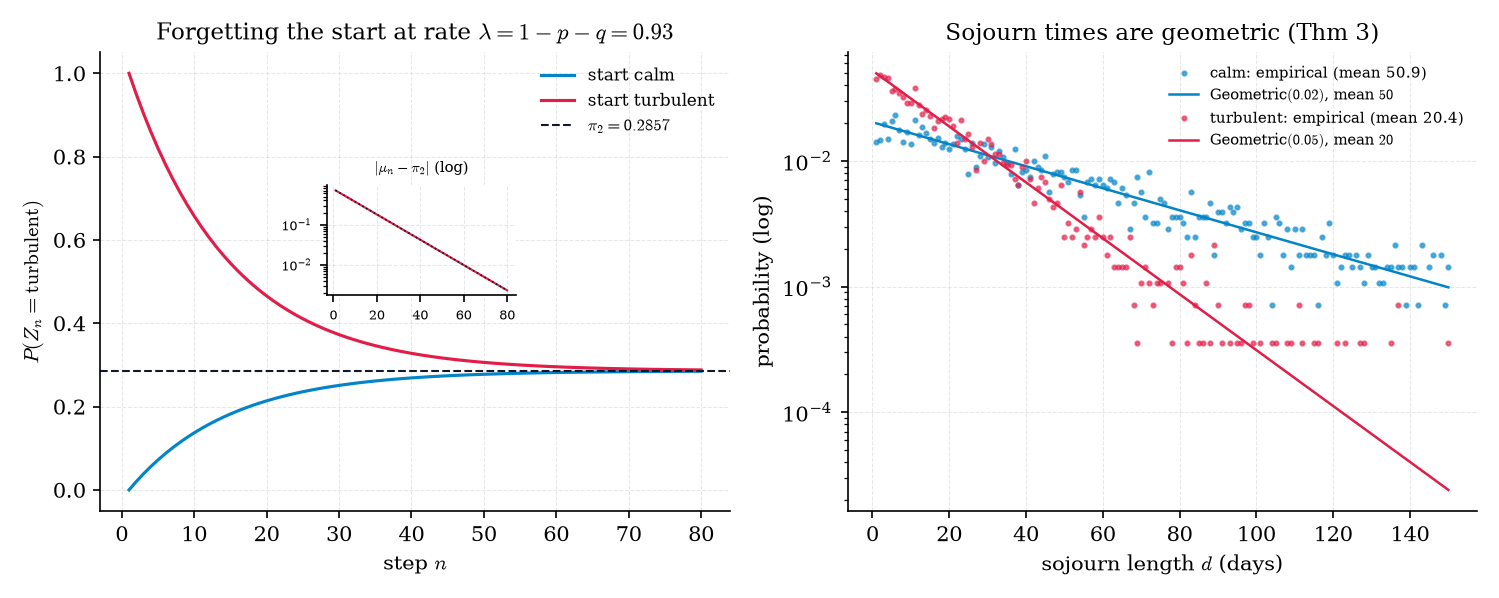
Figure 2. A two-state chain forgets its starting point at rate λ = 1 − p − q, and the time it spends in each state is geometric.
With states, the second-largest eigenvalue modulus of plays the role of : the chain forgets its starting point at roughly the rate , and is called the spectral gap. That is the finite-state face of a mixing-time bound, developed in formalML: random-walks . We won’t need more than the two-state case.
Requiring the next state to depend only on the current one costs less generality than it seems. A chain where the next state depends on the last states is a first-order chain on the possible blocks of states, so “first order” restricts only how big the state space is. The genuine restriction is Theorem 3: every state’s dwell time is geometric, so the most likely duration is always 1, whatever the mean. Regimes that tend to last about a month, or phonemes with a typical length, violate that. §34.9 Remark 21 gives the fix.
34.3 The hidden Markov model
Now we hide the chain and let it emit.
A hidden Markov model with states has parameters and satisfies:
(i) is a Markov chain with initial distribution and transition matrix ;
(ii) given the whole state sequence , the observations are independent, and has distribution , which depends only on the current state.
Here is a pmf or density, the emission distribution of state . In words: the state walks; at every step it emits one observation from its own distribution and otherwise leaves no trace. Categorical emissions have for symbols in a finite alphabet (the casino). Gaussian emissions have (the market).
Everything that follows rests on one theorem: the joint distribution factors along the chain, and the factorization makes the past and the future conditionally independent given the present state.
Under Definition 3, for every and every :
(i) the joint probability factors along the chain,
(ii) for each , the past block and the future block are conditionally independent given ; in particular ;
(iii) and .
Proof 3 Proof of Thm 4 (factorization and conditional independence) [show]
(i) Write . The first factor is by the chain rule and the Markov property. The second is by Definition 3(ii).
(ii) Group the factors of (i) by whether their indices are at most or greater than . Define
so that . The function touches the past only through . Fix and divide by , the sum of over every other variable. The conditional joint density of the two blocks given is then a function of the past block times a function of the future block. A joint density that factors this way is the product of its conditional marginals (Topic 2’s characterization of conditional independence, applied to densities), which is the claimed independence. The “in particular” statement applies it to the part of the future block.
(iii) Summing the future factors of (i) over and gives 1, so the joint of the prefix is the product (i) truncated at . Divide that truncated product by the same product with summed or integrated out. Every factor cancels except , because . The same argument at horizon , with summed out, leaves . — using the chain rule, the Markov property, and the factorization criterion for conditional independence.
Part (ii) is the remark Topic 2 made in passing (“in hidden Markov models, observations are conditionally independent given the hidden state”), now proved. It’s the only property of the model the algorithms will use: the current state screens off the past from the future.
In the casino, start the chain at its stationary distribution (fair, loaded). Take the rolls and the path . Theorem 4(i) multiplies one factor per edge and node of the path:
Summing this product over all paths gives the likelihood of the rolls, . That 8-term sum is the brute-force computation §34.4 replaces.
The factorization also tells us what an HMM’s observations look like marginally: what statistics they have once we sum the hidden states out.
Take a two-state HMM started at stationarity with Gaussian emissions, and write and for the mean and variance of state . Fix a lag . Given the whole state path, and are independent (Theorem 4), so their covariance comes entirely from the states. Conditioning on the path and using the tower property,
Now use the -step formula from Example 3:
Subtracting leaves times the variance of . For two states that variance is , so
The same argument applied to , with in place of , gives
In the market model the means barely differ (0.05 vs −0.10), so returns are nearly uncorrelated: the theoretical lag-1 autocorrelation is 0.0029. The second moments differ a lot (, ), so squared returns are strongly autocorrelated, decaying like . At lags the theory gives 0.1947, 0.1457, 0.0490; a 200,000-day simulation gives 0.1893, 0.1450, 0.0471, and the 1,000-day series of Example 1 gives 0.206, 0.124, 0.043. That is volatility clustering, produced by nothing more than a persistent hidden state. The model has no feedback from past returns to future variance; GARCH builds that feedback in directly, and Topic 35 fits it to this same data.
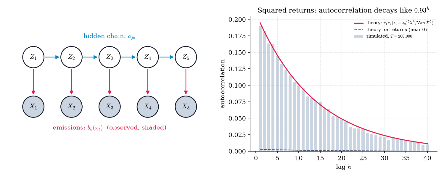
Figure 3. The HMM’s graph, and the volatility clustering it implies: the autocorrelation of squared observations decays like λ^h.
If every row of equals , the next state ignores the current one, the labels are i.i.d. draws from , and the HMM is exactly the Gaussian mixture of Topic 14’s EM appendix. Then and every autocovariance in Example 5 vanishes. The HMM’s extra content over a mixture is persistence: the cluster label at time predicts the label at time . The “No memory” preset in the simulator below makes this concrete. Mixtures and their EM are developed in formalML: clustering .
Figure 3’s directed graph encodes Theorem 4 by itself. Conditional independence (ii) is d-separation: every path from the past to the future passes through , and observing blocks it. Naive Bayes reads the same picture one time step at a time: one hidden class, many conditionally independent features. The HMM strings naive-Bayes models together along a Markov chain.
Try the generative model yourself. Raise the stay probabilities and the regimes lengthen, the sojourn histograms flatten into longer geometric tails, and the autocorrelation of the squared observations decays more slowly, along Example 5’s curve. The “No memory” preset keeps the marginal distribution and destroys the time structure.
34.4 Likelihood: the forward algorithm
The first of Rabiner’s problems is to compute : how probable is the observed sequence under the model? We need it to compare models, to fit them by maximum likelihood, and to flag anomalous sequences. By total probability over the hidden path,
a sum of terms, each a product from Theorem 4(i). For the 300 casino rolls that is paths. The sum is correct and useless. The way out is to organize it along time.
The forward variable is the joint probability of the observations so far and the current state,
The filtering distribution is : what we believe about the state now, having seen everything up to now and nothing after.
The forward variables satisfy and, for ,
Consequently , and computing it takes operations.
Proof 4 Proof of Thm 5 (forward recursion) [show]
The base case is Theorem 4(i) with . For , marginalize and apply the chain rule:
The first factor is . By Theorem 4(iii) the second is and the third is . Pull out of the sum. The likelihood is total probability over . For the cost, each of the steps computes sums of products. — using the chain rule and Theorem 4(iii).
The trellis makes the recursion visible. Each node holds , computed from the nodes of the previous column along the incoming edges. Every path through the trellis is still counted, but the paths that share a prefix share its arithmetic.
The forward algorithm costs about multiply-adds: 2,396 for the 300 casino rolls. Brute force costs about 6.1 × 10⁹². Both compute the same number. For the first 10 casino rolls (faces 1, 2, 5, 6, 4, 4, 2, 2, 1, 4), forward and brute-force enumeration of all paths both give −18.488737947800, identical to double precision.
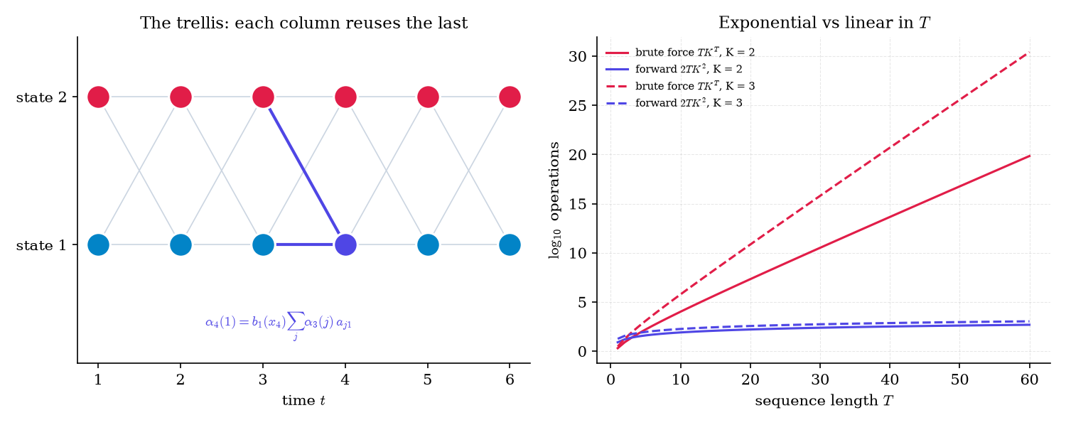
Figure 4. The forward algorithm reuses each column of the trellis instead of enumerating every path — linear in T instead of exponential.
There’s a numerical catch. Every is a probability of specific observations, so it shrinks geometrically in and soon falls below the smallest positive double. The fix normalizes each column, and the normalized column turns out to be exactly the quantity we wanted anyway.
Define with , and for
Then:
(i) , with ;
(ii) ;
(iii) .
Every normalized quantity lies in , so nothing underflows.
Proof 5 Proof of Thm 6 (scaling equals filtering) [show]
We prove (i) and (ii) together by induction on . At , and . Suppose . Substitute it into and use Theorem 5:
Summing over , , which is (i). Dividing, , which is (ii); its second equality is the definition of conditional probability. For (iii), the chain rule gives . — using Theorem 5 and the definition of conditional probability.
Read the two lines of the recursion as two steps. The sum is the prediction: where the state will be next, before seeing . Multiplying by and normalizing is the update: Bayes’ theorem with the new observation as data. The normalizer is how surprising was, and the log-likelihood is the total surprise.
Run the unscaled recursion of Theorem 5 on the 1,000-day market series in double precision. The raw becomes exactly 0 at t = 542; after that the “likelihood” is . The scaled recursion runs to the end without trouble and gives −1522.1208729, which matches an independent log-sum-exp implementation to 1.4 × 10⁻¹² (about 15 significant digits). Figure 5’s right panel is the filter itself: , jumping toward 1 at the first large return of each turbulent stretch.
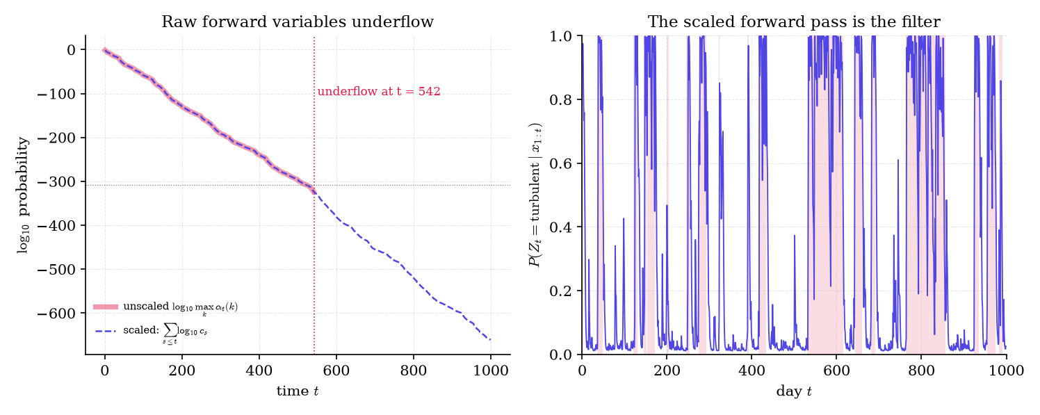
Figure 5. Unscaled forward variables underflow within a few hundred steps; the scaled recursion is the filter itself, and its scale factors multiply to the likelihood.
Scaling (Theorem 6) is one fix; the other is to run the recursion on log probabilities, replacing each sum with log-sum-exp, with . Both are exact. The site’s implementation uses scaling, because it produces the filtering distribution for free and keeps the backward pass of §34.5 in the same units.
Predict, then update: this is the same two-step recursion formalML’s sequential Monte Carlo page writes for general state spaces, with integrals over a continuous state in place of our sums over states. When the state is continuous and the model non-linear, those integrals have no closed form, and the bootstrap particle filter replaces the exact sum with a weighted sample of states ( formalML: sequential-monte-carlo ). The finite-state forward pass is the exact case it approximates. The same recursion appears in probabilistic programming: Stan and PyMC can’t sample discrete hidden states with gradient-based samplers, so they marginalize them out with exactly this forward pass ( formalML: probabilistic-programming ).
34.5 Smoothing: forward–backward (featured)
The filter answers “what is the state now, given the past?” Often the whole sequence is already in hand — a recorded utterance, a finished trading year, a sequenced genome — and the better question is “what was the state at time , given everything?” The answer conditions on the future too, and the future can only sharpen it.
The backward variable is the probability of the future observations given the current state,
The smoothing marginals are , the posterior probability of state at time given all the data, and , the posterior probability that the transition from to was .
The backward variables satisfy and, for ,
For every :
(i) , hence for every ;
(ii) ;
(iii) for .
With the scaled forward variables of Theorem 6 and , the same formulas hold with in place of : the denominator disappears from (ii), so (elementwise product), and replaces in (iii).
Proof 6 Proof of Thm 7 (forward–backward) [show]
Backward recursion. by convention: an empty block of future observations has probability 1. For , marginalize :
The first factor is , and the second is by Theorem 4(iii). For the third, Theorem 4(ii) at time says is conditionally independent of given , so the factor is .
(i). By the chain rule,
The first factor is . By Theorem 4(ii) the conditioning on can be dropped from the second, leaving . Summing over gives the second claim, which is a free consistency check: the product summed over states is the same number at every .
(ii) is (i) divided by , by the definition of conditional probability.
(iii). Expand the joint with the chain rule in time order:
Each conditional factor is simplified by Theorem 4(ii)–(iii) exactly as in the backward step: the next state depends only on , the emission only on , and the future block only on . The factors are , , and ; divide by .
Scaled version. By Theorem 6(ii), , and by definition . So
by Theorem 6(iii) and (ii) above. In (iii), the scale factors in the denominators of and multiply to , which gives the stated . The scaled backward recursion is . — using the chain rule, Theorem 4(ii)–(iii), and Theorem 6.
Geometrically, the forward pass carries evidence across the trellis from left to right and the backward pass carries it from right to left. At each column they meet, and the posterior is their elementwise product. Two passes of each give all marginals and all the pairwise transition marginals, which is exactly what learning will need (§34.7).
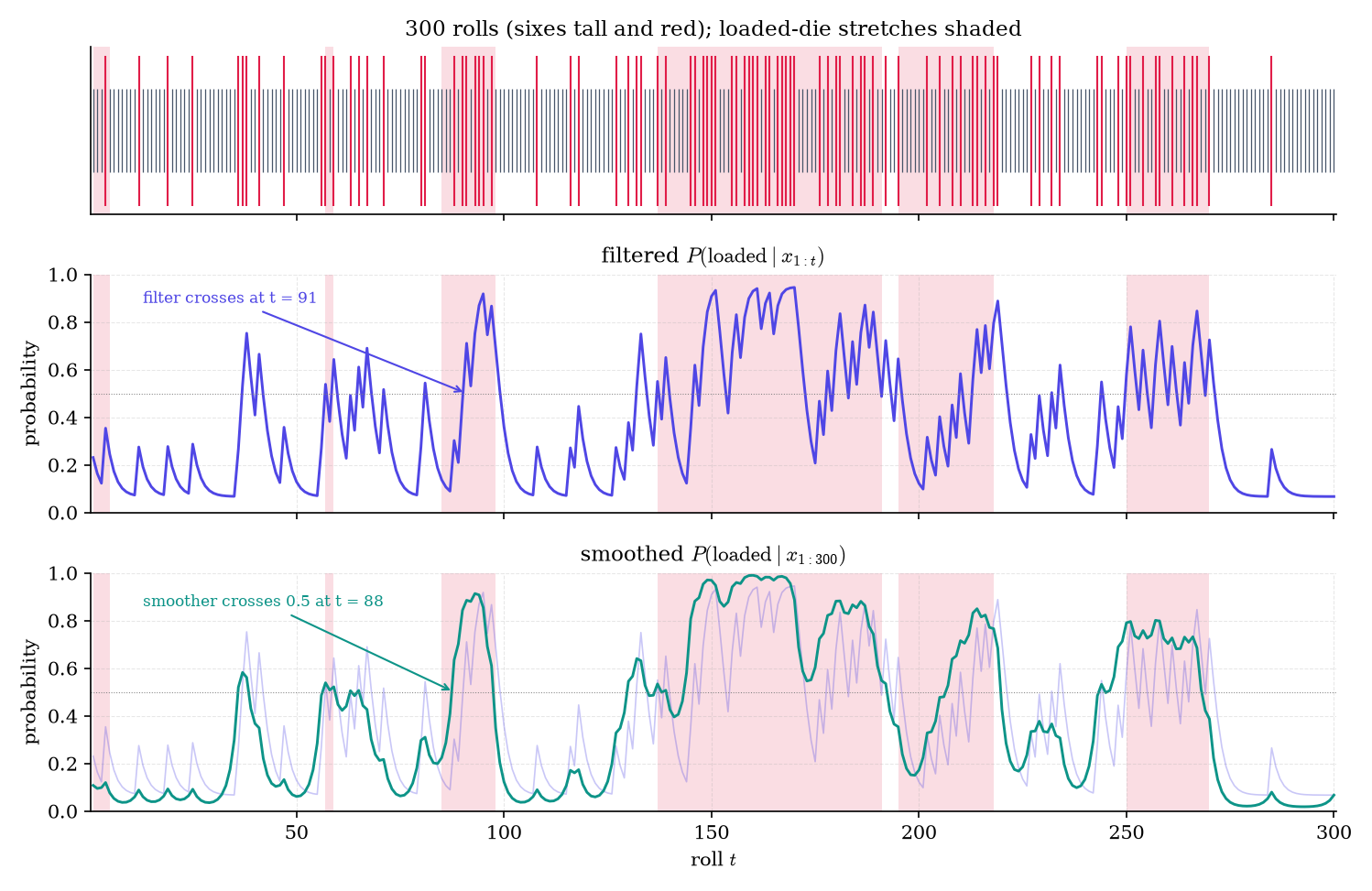
Figure 6. Forward–backward on the dishonest casino. The smoother sees the end of each loaded run and reacts before the filter can.
The explorer below runs both passes on a simulated sequence. The three heatmap rows are (the filter), (rescaled per column for display), and their product . Move the cursor to the start of a loaded run and watch the backward message arrive before the forward message has caught on. The readout confirms Theorem 7(i) at every step: . The switching-rate slider changes only the transition matrix used for inference: tell the model to expect fewer switches and smoothing borrows evidence from farther away.
On the 300 casino rolls (loaded 40.7% of the time), threshold each posterior at 0.5 and compare with the truth. The filter labels 75.7% of rolls correctly and the smoother 85.0%. The mean log-loss of the probabilities against the true states falls from 0.478 to 0.354. At the loaded run that starts at roll 85, the smoother crosses 0.5 at roll 88 and the filter only at roll 91: the smoother has already seen the run of sixes that follows. The filter also raises more false alarms. A cluster of sixes near roll 38 pushes the filtered probability to 0.75, and the smoother, seeing the fair rolls that come after, holds it to 0.58.
On the 1,000-day market series, the true regime path switches 37 times. Thresholding the filtered probability of turbulence at 0.5 switches 53 times: the filter flickers whenever a single large calm-day return looks turbulent. The smoother switches 29 times. Its accuracy is 94.8% against the filter’s 89.6%.
The ML reading is a warning. A backtest that conditions trading decisions on smoothed regimes uses information from the future: at day the smoother has seen days . A live system gets only the filter. Using where belongs is a textbook leakage bug, and the 5-point accuracy gap above is roughly how much it can flatter a backtest.
The filter is online and the smoother is offline. In between is the fixed-lag smoother : wait steps, then commit to a belief about time . It costs a delay of and recovers most of the smoother’s accuracy when is a few multiples of the typical regime length. Which one to use is a latency decision, not a statistical one.
Forward–backward is belief propagation on the HMM’s chain-shaped graph. The forward variables are messages passed left to right and the backward variables are messages passed right to left. On any tree-shaped graph the same messages give exact marginals. On graphs with loops, running them anyway gives “loopy” belief propagation, an approximation that works surprisingly well in practice. The chain is the cleanest case: every message is exact and the whole computation is two sweeps.
34.6 Decoding: the Viterbi algorithm
Smoothing gives a probability for each state at each time. Often we need a single answer: one label per time step, a transcription, a segmentation, a gene annotation. There are two natural ways to get one, and they answer different questions.
The MAP path is the single most probable hidden path,
Posterior (pointwise) decoding picks the most probable state at each time separately: . The first is “the single most probable story”; the second is “the most probable state at each moment, considered one moment at a time.”
Posterior decoding is a byproduct of forward–backward. The MAP path needs one more recursion: the forward recursion with the sum replaced by a maximum.
Let , the probability of the best path that ends in state at time , with . Then for
Set and backtrack with for . Then maximizes over all paths, and . The cost is time and memory for the back-pointers .
Proof 7 Proof of Thm 8 (Viterbi) [show]
Recursion. By Theorem 4(i), the joint probability of a prefix factors as
Maximize over in two stages: first over with held fixed, then over . In the first stage the factor doesn’t depend on , and for a nonnegative constant , . So the inner maximum is , and maximizing over gives the recursion. The maximizing is the back-pointer .
Backtracking. Define, for every state and time , the backtracked path ending in : and for . We show by induction on that this path attains , meaning , for every . At it is the definition. Suppose it holds at for every state. With , the path is followed by , so by the factorization above and the induction hypothesis for ,
the last step being the definition of . At , the backtracked path from is exactly , and maximizes , so . Finally, and doesn’t depend on , so also maximizes the posterior. — using Theorem 4(i) and the fact that maximization commutes with multiplication by a nonnegative constant (Bellman’s principle of optimality).
The two decoders usually agree. They can disagree sharply, and the disagreement can be disqualifying.
Take three states with two structural zeros, : the chain can’t jump between states 1 and 3 without passing through 2. Let
with a uniform starting distribution and binary emissions, for . Observe . Forward–backward gives these smoothed marginals (rows are times; the largest entry in each row is in bold):
| 1 | 0.307 | 0.316 | 0.377 |
| 2 | 0.367 | 0.294 | 0.339 |
| 3 | 0.413 | 0.286 | 0.301 |
| 4 | 0.458 | 0.270 | 0.272 |
| 5 | 0.555 | 0.140 | 0.305 |
Posterior decoding reads off , and its first step is the forbidden transition . So : the “most probable state at each time” assembles into a path the model says cannot happen. Viterbi returns , with posterior probability 0.148. Enumerating all paths confirms both answers.
The lesson: when the transition structure carries hard constraints — a gene grammar where exons and introns alternate, a phoneme graph that fixes the order of sounds in a word, a protocol state machine — decode with Viterbi. Pointwise decoding optimizes each label without checking that the labels fit together.
The two decoders optimize different losses. Posterior decoding maximizes the expected number of correctly labeled rolls under the model; Viterbi maximizes the probability of getting the whole path right. On the 300 casino rolls, the model’s own expected accuracy (the average of at the decoded state) is 0.800 for posterior decoding and 0.777 for Viterbi, as the theory says it must be.
On this particular realization the realized accuracies flip: Viterbi labels 88.7% of rolls correctly and posterior decoding 85.0%. That isn’t a contradiction. An expectation guarantee is a statement about the average over sequences the model could have produced, not a promise about every sequence.
Where the decoders differ reliably is segment structure. The true path switches dice 11 times. Viterbi’s path switches 6 times; it merges short excursions into the surrounding segment because a switch costs a factor of or in path probability. Posterior decoding switches 24 times, flickering wherever hovers near 0.5. As a whole path, Viterbi’s has −21.07, against −55.03 for the posterior-decoded path.
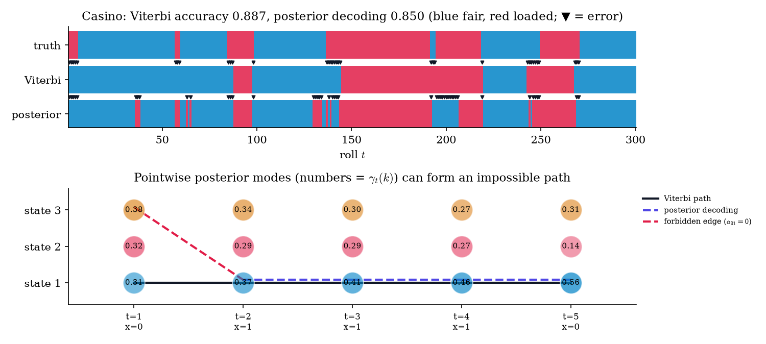
Figure 7. Viterbi’s single best path versus the sequence of most probable states. The second can be a path the model forbids.
In the decoder below, click any roll to cycle its face. Engineer a run of sixes and watch both decoders respond: posterior decoding flips the affected rolls one at a time, while Viterbi waits until the run is long enough to pay for two switches. The second scenario is Example 10.
The forward algorithm combines edges with : multiply along a path, add across paths. Viterbi uses . In log space Viterbi becomes : each edge has a length , and is the shortest path through the trellis (FOR1973). That is Bellman’s dynamic programming, and it’s why Viterbi in log space never needs scaling: sums of logs don’t underflow.
For three decades, speech recognizers were HMMs: one small chain per phoneme, phoneme chains joined into word chains by a pronunciation dictionary, and Viterbi over the resulting graph to transcribe audio. Beam search in modern sequence models is Viterbi made approximate: the state space (every possible prefix) is too large to sweep exactly, so the search keeps only the best few partial paths. And the CTC loss used to train speech and handwriting recognizers (GRA2006) is a forward–backward sum over all alignments of a label sequence to an input sequence.
34.7 Learning: Baum–Welch as EM
So far the parameters were known. In practice we have only observations, and must learn from them. Maximum likelihood is the natural target, and §34.4 computes the likelihood, but maximizing it directly is awkward: is a log of a sum over paths. Topic 14’s EM appendix previewed the general strategy for likelihoods with latent variables: alternate between guessing the latent variables and maximizing as if the guesses were data. It stated without proof that each iteration increases the likelihood. Here we prove it, then work out what EM does for an HMM.
The complete-data log-likelihood is the log-likelihood we would have if the hidden path were observed,
The EM objective averages it over the posterior of the path under the current parameter :
The E-step computes (in practice, the posterior expectations it needs), and the M-step sets .
Let for observed and latent (finitely many values, or densities), with wherever . For any :
Hence if maximizes , or merely increases it, then .
Proof 8 Proof of Thm 9 (EM ascent) [show]
For any with , Bayes’ theorem gives . The left side doesn’t depend on , so average both sides over :
The same identity holds at . Subtracting the two,
The second bracket is , the Kullback–Leibler divergence between the two posteriors over paths (Topic 24 §24.3). It is nonnegative by Jensen’s inequality applied to the concave , with all expectations over :
Dropping the nonnegative second bracket gives the inequality. If the M-step makes the first bracket nonnegative, the likelihood doesn’t decrease. — using Bayes’ theorem, Jensen’s inequality, and the nonnegativity of KL divergence.
The proof also shows when EM stops. Equality forces both brackets to zero, so at a fixed point maximizes , and if is differentiable then at . Since is minimized at , the gradients match there, so too. WU1983 gives the conditions under which the iterates actually converge to such stationary points. That is the “equality only at a stationary point” clause in Topic 14’s appendix. A stationary point need not be the global maximum, and for HMMs it often isn’t (Example 13).
For an HMM, the M-step has a closed form, and the E-step is forward–backward.
Let and be the smoothing marginals computed by Theorem 7 under . Then is maximized over by
and, for categorical emissions, ; for Gaussian emissions,
Proof 9 Proof of Thm 10 (Baum–Welch M-step) [show]
Decomposing Q. Take the log of Theorem 4(i) at and write each term with indicators:
Take the expectation over . The expected indicators are exactly , and :
The three groups involve disjoint parameters, so we maximize each one separately.
A weighted-log lemma. For weights with , the maximum of over probability vectors is attained at . To see it, form the Lagrangian ( formalCalculus: The Gradient ). Setting gives , and the constraint gives . The objective is concave (a nonnegative combination of the concave functions ) on the convex set of probability vectors, so this stationary point is the global maximum.
Initial distribution: the lemma with and .
Transitions: the entries for different sit in separate terms and are constrained separately (each row sums to 1), so apply the lemma row by row with . Its total is , because summing the pairwise marginal over the second state gives the single marginal.
Categorical emissions: the lemma for row with .
Gaussian emissions: for each , is a Normal log-likelihood with weights , where is the Normal density. Setting the -derivative to zero gives the weighted mean. Setting the -derivative to zero at gives the weighted variance. This is Topic 14’s Normal MLE with weights, and the same concavity argument, in the parameters , makes it the maximum. — using Theorem 4(i), Theorem 7, Lagrange multipliers, and the Normal MLE (Topic 14).
The updates have an intuitive reading. The new transition probability is the expected number of transitions divided by the expected number of visits to , with expectations under the current posterior. The new emission parameters are the usual estimates, each observation weighted by how likely it is to have come from that state. If we could see the path, these would be counts. EM uses expected counts instead.
Fit a two-state Gaussian HMM to the 1,000-day market series (rounded to 6 decimals, the fixture the site’s tests use). Initialize deterministically with one-dimensional k-means: centers −1.049 and 0.843, SDs 0.996 and 0.911, so neither starting state looks like either true regime. Baum–Welch converges () in 25 iterations, and every iteration increases the log-likelihood; the smallest increase is . Fitted against true values (calm, turbulent):
- standard deviations 0.711, 2.073 (true 0.7, 2.0);
- stay probabilities 0.9717, 0.9415 (true 0.98, 0.95);
- means 0.036, −0.040 (true 0.05, −0.10).
The fitted log-likelihood −1519.40 exceeds the true parameters’ −1522.12, as a maximum-likelihood fit should in-sample. The means are the weakest estimates: 1,000 days barely pin down a 0.15-point gap in means under this much noise, while the volatilities and persistences are well identified. One more detail: collapses onto the state of day 1. A single sequence contains a single draw of , so the initial distribution is essentially unestimable without several sequences.
Now take a three-state market (calm, normal, crisis: means 0.06, 0, −0.3 and SDs 0.5, 1.0, 3.0), simulate 1,500 days, and run Baum–Welch from 50 random starting points. Each start draws its transition rows from a Dirichlet(1) distribution (uniform over probability vectors), its means from the data, and its SDs between 0.5 and 1.5 times the sample SD. The runs end at 6 distinct optima, separated by more than 0.1 in log-likelihood. The best, −1951.52, is reached by 88% of the starts; the worst is −1992.86. The true parameters score −1956.31, below the best fit (in-sample again). Every run climbs monotonically, as Theorem 9 guarantees, but they climb different hills.
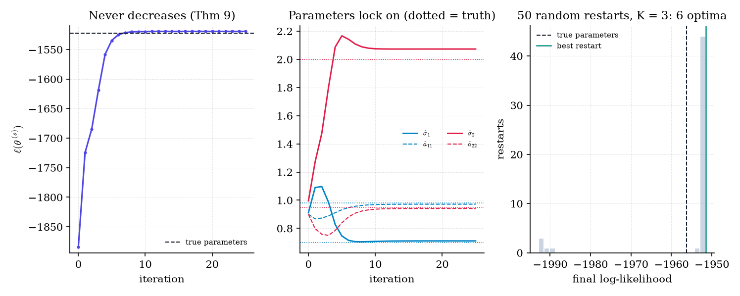
Figure 8. Baum–Welch never decreases the likelihood, but where it stops depends on where it starts.
The fitter below runs EM step by step. Watch the trace climb and the fitted densities settle onto the histogram. Then fit with more states than the truth, or press “New random init” a few times and run each to convergence: the restart tally collects the final log-likelihoods and reproduces Example 13’s spread. A red badge would appear if the log-likelihood ever decreased. It shouldn’t, and that is Theorem 9 checked live.
Permuting the state labels of — swapping which state we call “1” and which “2”, and permuting , the rows and columns of , and the emissions to match — gives exactly the same likelihood. So the likelihood has at least equivalent maxima, and the labels in a fit mean nothing until we fix a convention after fitting, such as sorting the states by emission mean or by variance. For a single maximum-likelihood fit that’s a cosmetic step. For Bayesian HMMs, whose posterior is multimodal by this symmetry, it’s a real problem for MCMC summaries.
As with Gaussian mixtures, the HMM likelihood is unbounded: put one state’s mean exactly on one observation and let its variance shrink to zero, and that observation’s density, and with it the likelihood, goes to infinity. EM can drift toward such a degenerate solution on small data. The standard defenses are a variance floor (the site’s implementation floors each variance at times the sample variance) or a prior on the variances, which turns the fit into MAP estimation.
Baum and colleagues proved the monotonicity of this algorithm for HMMs in 1970 (BAU1970), seven years before Dempster, Laird and Rubin named the general EM algorithm and proved Theorem 9 in general (DEM1977). The NPMLE grid algorithm of Topic 33 §33.6 is another instance, with the prior’s weights in the role of .
Fisher’s identity says the gradient of the log-likelihood is the posterior expectation of the complete-data gradient: . Equivalently, automatic differentiation through the scaled forward pass of Theorem 6 gives the exact gradient of . That’s how HMM layers sit inside neural networks and get trained by stochastic gradient descent along with everything else, with no M-step at all.
Put priors on , the rows of (Dirichlet), and the emission parameters (Normal–inverse-gamma, say), and sample the posterior by Gibbs sampling (Topic 26 §26.3), alternating two blocks. Given , draw the whole path at once by forward-filtering backward-sampling: run the filter, sample from , then sample each earlier state given the one after it (SCO2002). Given the path, draw from its conjugate full conditionals (Topic 25), which use the same counts as the M-step, now as data in a conjugate update.
34.8 Identifiability and choosing the number of states
Two questions remain before an HMM fit can be trusted: are the parameters determined by the data at all, and how many states should the model have?
Suppose the hidden chain is stationary, irreducible and aperiodic, the transition matrix has full rank, and the emission distributions are linearly independent. If two parameter values and induce the same distribution of , then is obtained from by a permutation of the state labels.
So label switching (Remark 13) is the only ambiguity, and three consecutive observations already carry all the information about . The proof (GAS2016, building on Kruskal’s uniqueness theorem for three-way arrays, as ALL2009 does for finite emission alphabets; PET1969 is the classical finite-alphabet result) is outside our spine. Notice what the conditions exclude: two states with the same emission distribution, or a transition matrix with linearly dependent rows (the “no memory” case of Remark 5 has rank 1), break identifiability.
Simulate 2,000 days from the three-state market of Example 13 and fit states, keeping the best of 10 starts (one k-means and nine random) for each . A Gaussian HMM with states has free parameters: the initial distribution, the transition rows, and a mean and variance per state. The criteria from Topic 24 are and :
| BIC | AIC | |||
|---|---|---|---|---|
| 1 | −3312.57 | 2 | 6640.34 | 6629.13 |
| 2 | −2437.92 | 7 | 4929.05 | 4889.84 |
| 3 | −2388.79 | 14 | 4884.00 | 4805.59 |
| 4 | −2384.22 | 23 | 4943.26 | 4814.44 |
| 5 | −2380.09 | 34 | 5018.61 | 4828.18 |
Both criteria pick K = 3, the truth. AIC’s curve is much flatter beyond the truth (+9 at , against +59 for BIC), the familiar pattern of AIC’s lighter penalty overfitting more readily.
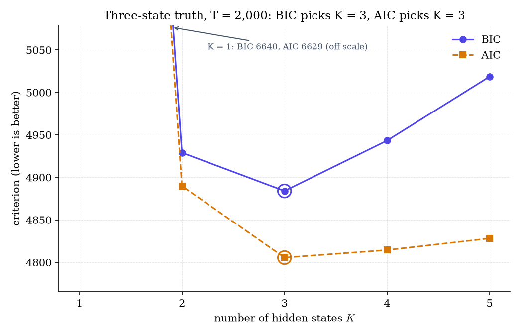
Figure 9. Information criteria over the number of hidden states.
BIC’s derivation (Topic 24 §24.4) is a Laplace approximation that needs a regular model: an interior maximum and an invertible Fisher information. An HMM with more states than the truth is not regular. The extra states can duplicate a true state or go unused, the parameters are non-identifiable (Theorem 11’s conditions fail), and the Fisher information is singular. In practice BIC still tends to choose well, as in Example 14, but the guarantee is gone. The robust alternative is held-out predictive log-likelihood on contiguous blocks of the sequence. Randomly scattered held-out points leak information through the Markov dependence, because their neighbors are in the training set.
Under regularity conditions, the HMM MLE is consistent and asymptotically Normal, with a Fisher information defined through the stationary chain (BIC1998). It’s the time-series analogue of the i.i.d. result in Topic 14 §14.5. The proof needs the forgetting property of Theorem 2, applied to the filter rather than the chain.
34.9 Beyond finite states: the Kalman filter and continuous time
Nothing in Theorem 4 needed the state space to be finite. Replace sums over states by integrals and every recursion in this topic still holds; the problem is that the integrals rarely have closed forms. There is one great exception.
A linear-Gaussian state-space model has a vector-valued hidden state and vector observations,
with state noise , observation noise , and initial state , all mutually independent. The matrix moves the state forward, maps the state to what we observe, and are the noise covariance matrices. It’s an HMM with a continuous state: Definition 3 with a Gaussian transition kernel and Gaussian emissions, and Theorem 4’s factorization holds verbatim with densities.
The miracle of this model is that every filtering distribution stays Gaussian, so the filter only has to track a mean and a covariance.
Under Definition 8, suppose . Then:
Predict. , with and .
Update. With innovation , innovation covariance , and gain ,
Likelihood. , so , where is the multivariate Normal density: the continuous-state analogue of Theorem 6(iii).
Starting from (take , ), induction makes every filtering distribution Gaussian with these moments.
Proof 10 Proof of Thm 12 (Kalman filter) [show]
Predict. , and is independent of by Definition 8’s independence assumptions and Theorem 4(ii), whose proof applies verbatim to densities. So, conditionally on , is an affine map of a Gaussian vector plus an independent Gaussian vector, hence Gaussian (Topic 8, §8.3: affine maps and sums of independent Normals stay Normal). Its mean is and its covariance , by the covariance rules for affine maps and independent sums.
Joint of state and observation. with independent of . So, conditionally on , the pair is jointly Gaussian with means and covariance blocks
The cross-covariance uses . The marginal of given the past is the likelihood claim.
Update. Apply the conditional MVN formula (Topic 8 §8.4 Thm 3): for a jointly Gaussian pair, and . Take block 1 to be and block 2 to be :
where the last step uses . — using Topic 8 §8.3 (affine maps of Normals), §8.4 Thm 3 (conditional MVN), and Theorem 4(ii) for densities.
The structure is Theorem 6’s, line for line. The predict step pushes the belief through the dynamics, and the update step conditions on the new observation. The gain decides how far the new observation moves the estimate: close to 1 when the prediction is uncertain relative to the observation noise, close to 0 when the observation is the noisy one. (The subscript always distinguishes the gain from the number of states .)
The simplest state-space model is a random walk observed with noise: , state-noise variance , observation-noise variance . The scalar Kalman recursions are
Combining them gives a recursion for the predicted variance alone (the Riccati recursion):
It converges to a fixed point , which solves , that is, :
Once the gain has settled, the filter is : an exponentially weighted moving average with smoothing weight . The weight that practitioners usually tune by hand is derived here from the signal-to-noise ratio .
With and : 0.370156 and 0.270156. Starting from a vague prior (so ), the gain is within of from step 22 on, and after step 20 the exponential smoother and the Kalman mean never differ by more than 3.1 × 10⁻⁴. The filter tracks the hidden level with error 0.515 (root mean square), against 0.997 for the raw observations.
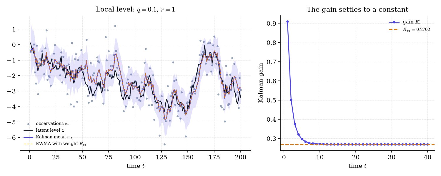
Figure 10. The Kalman filter for a local-level model. Its gain settles to a constant, and the filter becomes an exponentially weighted moving average.
Time itself can be made continuous too.
A continuous-time Markov chain on is governed by a generator matrix whose off-diagonal entries are jump rates and whose rows sum to 0. Its transition matrices are , the matrix exponential, and the time it stays in state is : the continuous twin of Theorem 3. A Markov-modulated Poisson process (MMPP; FIS1993) is an HMM in continuous time: events arrive as a Poisson process whose rate is set by the hidden chain.
The transition matrices of a continuous-time chain solve with , a linear system of first-order ODEs ( formalCalculus: First-Order ODEs & Existence Theorems ), whose solution is . Sampling a continuous-time chain every time units gives a discrete-time chain with , which is how irregularly timed data enter the discrete framework: each gap gets its own transition matrix. In ML systems an MMPP is a natural model for bursty event streams, such as requests to a service, clicks in a session, or trades in a book, where the arrival rate itself switches between regimes.
Theorem 3 and Remark 4 flagged the HMM’s built-in assumption that every state’s duration is geometric. Hidden semi-Markov models (YU2010) give each state an explicit duration distribution (Poisson, negative binomial, or anything else) and let the chain jump only when the duration expires. The forward recursion gains a sum over durations, costing for maximum duration , and segment lengths stop being forced to have their mode at 1.
The Kalman update is exact only because Gaussian conditioning has a closed form. With nonlinear dynamics or observations, the extended Kalman filter linearizes the model around the current estimate and the unscented filter propagates a few carefully chosen points. Particle filters give up on closed forms entirely and approximate the filtering distribution by weighted samples (formalML’s formalML: sequential-monte-carlo , §6). That page cites the Kalman filter of Theorem 12 as the exact baseline its particle filter generalizes.
34.10 Connections to ML and the road ahead
One structure did all the work in this topic: a hidden Markov chain with observations that depend only on the current state (Theorem 4). It turned three exponential problems into linear-time sweeps over one trellis. Summing over the trellis gives the likelihood and the filter (§34.4); summing forward and backward gives the smoother (§34.5); maximizing gives Viterbi (§34.6); and iterating smoothing with expected-count updates gives Baum–Welch (§34.7). The same recursion with a Gaussian state is the Kalman filter (§34.9), and with weighted samples in place of sums it’s the particle filter. Four places where this machinery runs in practice:
GMM-HMM acoustic models, with a Gaussian mixture as each state’s emission distribution, were the core of speech recognition for decades. Hybrid systems replaced the emission model with a neural network that outputs state posteriors and kept the HMM for the time structure. In language, HMM part-of-speech taggers gave way to the linear-chain conditional random field (LAF2001). The CRF models directly instead of modeling how the words were generated, but keeps the chain structure, so its marginals and its best path come from exactly the forward–backward and Viterbi recursions of §34.5–§34.6. A CRF layer on top of a neural encoder is still a standard choice for named-entity recognition.
The casino is a cartoon of a real problem. CpG islands are stretches of DNA where the dinucleotide CG is unusually frequent, and a two-state HMM over the four-letter alphabet finds them exactly as Example 8 finds the loaded die (DUR1998 §3.3). Gene finders use HMMs whose states encode exons, introns and the boundaries between them, a transition structure with hard constraints of the kind Example 10 warns about. Profile HMMs model protein families with one match, insert and delete state per alignment column; database searches for distant relatives of a protein run the forward algorithm against thousands of them.
Modern linear state-space layers such as S4 (GU2022) and Mamba (GU2023) run the recurrence : Definition 8’s state equation with learned matrices and no noise model. They aren’t probabilistic filters, since nothing is conditioned on, but they share the linear-in- scan structure that made Theorem 5 practical, and their designers lean on the same linear-systems theory as the Kalman filter. In econometrics, Hamilton’s Markov-switching model (HAM1989) uses the HMM directly as a time-series model: a regression whose coefficients switch with a hidden business-cycle regime, fit by exactly the filter of Theorem 6.
This topic opens the time-series track with the latent-state view. Future Track 9 topics build out from here: Kalman smoothing and EM for linear-Gaussian models (the continuous-state counterparts of §34.5 and §34.7), autoregressive and ARIMA models and the Wold decomposition, conditional heteroskedasticity (GARCH) as the observation-driven alternative to Example 5’s state-driven volatility, and spectral methods for stationary series.
References
- Rabiner, Lawrence R. (1989). A Tutorial on Hidden Markov Models and Selected Applications in Speech Recognition. Proceedings of the IEEE, 77(2), 257–286.
- Baum, Leonard E., and Ted Petrie. (1966). Statistical Inference for Probabilistic Functions of Finite State Markov Chains. Annals of Mathematical Statistics, 37(6), 1554–1563.
- Baum, Leonard E., Ted Petrie, George Soules, and Norman Weiss. (1970). A Maximization Technique Occurring in the Statistical Analysis of Probabilistic Functions of Markov Chains. Annals of Mathematical Statistics, 41(1), 164–171.
- Viterbi, Andrew J. (1967). Error Bounds for Convolutional Codes and an Asymptotically Optimum Decoding Algorithm. IEEE Transactions on Information Theory, 13(2), 260–269.
- Forney, G. David, Jr. (1973). The Viterbi Algorithm. Proceedings of the IEEE, 61(3), 268–278.
- Dempster, A. P., N. M. Laird, and D. B. Rubin. (1977). Maximum Likelihood from Incomplete Data via the EM Algorithm. Journal of the Royal Statistical Society, Series B, 39(1), 1–22.
- Wu, C. F. Jeff. (1983). On the Convergence Properties of the EM Algorithm. Annals of Statistics, 11(1), 95–103.
- Petrie, Ted. (1969). Probabilistic Functions of Finite State Markov Chains. Annals of Mathematical Statistics, 40(1), 97–115.
- Allman, Elizabeth S., Catherine Matias, and John A. Rhodes. (2009). Identifiability of Parameters in Latent Structure Models with Many Observed Variables. Annals of Statistics, 37(6A), 3099–3132.
- Gassiat, Elisabeth, Alice Cleynen, and Stéphane Robin. (2016). Inference in Finite State Space Non Parametric Hidden Markov Models and Applications. Statistics and Computing, 26(1–2), 61–71.
- Bickel, Peter J., Ya’acov Ritov, and Tobias Rydén. (1998). Asymptotic Normality of the Maximum-Likelihood Estimator for General Hidden Markov Models. Annals of Statistics, 26(4), 1614–1635.
- Kalman, Rudolph E. (1960). A New Approach to Linear Filtering and Prediction Problems. Journal of Basic Engineering, 82(1), 35–45.
- Hamilton, James D. (1989). A New Approach to the Economic Analysis of Nonstationary Time Series and the Business Cycle. Econometrica, 57(2), 357–384.
- Cappé, Olivier, Eric Moulines, and Tobias Rydén. (2005). Inference in Hidden Markov Models. Springer.
- Zucchini, Walter, Iain L. MacDonald, and Roland Langrock. (2016). Hidden Markov Models for Time Series: An Introduction Using R (2nd ed.). Chapman & Hall/CRC.
- Durbin, Richard, Sean R. Eddy, Anders Krogh, and Graeme Mitchison. (1998). Biological Sequence Analysis: Probabilistic Models of Proteins and Nucleic Acids. Cambridge University Press.
- Norris, J. R. (1997). Markov Chains. Cambridge University Press.
- Särkkä, Simo. (2013). Bayesian Filtering and Smoothing. Cambridge University Press.
- Bishop, Christopher M. (2006). Pattern Recognition and Machine Learning. Springer.
- Scott, Steven L. (2002). Bayesian Methods for Hidden Markov Models: Recursive Computing in the 21st Century. Journal of the American Statistical Association, 97(457), 337–351.
- Fischer, Wolfgang, and Kathleen Meier-Hellstern. (1993). The Markov-Modulated Poisson Process (MMPP) Cookbook. Performance Evaluation, 18(2), 149–171.
- Yu, Shun-Zheng. (2010). Hidden Semi-Markov Models. Artificial Intelligence, 174(2), 215–243.
- Lafferty, John, Andrew McCallum, and Fernando C. N. Pereira. (2001). Conditional Random Fields: Probabilistic Models for Segmenting and Labeling Sequence Data. In Proceedings of the 18th International Conference on Machine Learning (ICML 2001), 282–289.
- Graves, Alex, Santiago Fernández, Faustino Gomez, and Jürgen Schmidhuber. (2006). Connectionist Temporal Classification: Labelling Unsegmented Sequence Data with Recurrent Neural Networks. In Proceedings of the 23rd International Conference on Machine Learning (ICML 2006), 369–376.
- Gu, Albert, Karan Goel, and Christopher Ré. (2022). Efficiently Modeling Long Sequences with Structured State Spaces. International Conference on Learning Representations (ICLR 2022).
- Gu, Albert, and Tri Dao. (2023). Mamba: Linear-Time Sequence Modeling with Selective State Spaces. arXiv preprint arXiv:2312.00752.